Balanced Realization and Balanced Truncation — balance • rationalmatrices

Compute a balanced realization or a balanced truncated statespace realization of a rational matrix in statespace form.

Usage

balance(
  obj,
  gr,
  tol = 10 * sqrt(.Machine$double.eps),
  s0 = NULL,
  truncate = TRUE
)

Arguments

obj: (stsp object) rational matrix in statespace form.
gr: a list with two components P and Q which contain two Grammians. These Grammians may e.g. be computed with grammians.
tol: a tolerance parameter used for the determination of the rank $PQ$. If s0 = NULL then the procedure estimates the rank of $PQ$ and sets s0 equal to this estimate. If s0 is given, then tol is ignored.
s0: determines the size of the two diagonal blocks of transformed Grammians $P$, $Q$, respectively (for truncate = TRUE the statespace dimension of the balanced truncated statespace realization.
truncate: (boolean) If true then the balanced truncated model is returned.

Value

A list with components

obj: (stsp object) represents the balanced (truncated) statespace realization.
T,Tinv: the state transformation and the inverse state transformation matrix. Note that for the case truncate=TRUE the matrix T is an s0 x s matrix and Tinv is of dimension s x s0.
P,Q: the transformed (and truncated) Grammians.
sigma: the vector of singular values of the matrix $(P^{1/2}Q^{1/2})$.

Details

Let $P,Q$ denote the controllability and the observability Grammian of a statespace realization $$K(z) = C(Iz^{-1} - A)^{-1}B +D$$ of a rational matrix $K(z)$ with statespace dimension $s$. The matrix $PQ$ is diagonalizable and the eigenvalues are real and non negative. Let $\sigma_1^2 \geq \cdots \geq \sigma_s^2 \geq 0$ denote the eigenvalues of $PQ$ and suppose that $PQ$ has rank $k\leq s$, i.e. $\sigma_i=0$ for $i>k$. Then there exists a statespace transformation $T$ which renders both Grammians into diagonal form and furthermore we have $p_{ii}=q_{ii}=\sigma_i$ for the first $k$ diagonal entries of the (transformed) Grammians.

The (non zero) $\sigma_i$'s are equal to the (non zero) singular values of the Hankel matrix of the impulse response coefficients of $K$ and hence are called Hankel singular values. These singular values are also the singular values of the product $P^{1/2}Q^{1/2}$ where $P^{1/2}$ and $Q^{1/2}$ denote "square roots" of the Grammians $P$ and $Q$ respectively.

The procedure balance(obj,...) computes a somewhat simplified "balanced" form where the transformed Grammians $P,Q$ are block diagonal with two diagonal blocks of dimension $s_0$ and $s_1 = s - s_0$ respectively. The two upper, left blocks of $P$ and $Q$ are diagonal and the diagonal entries are $p_{ii}=q_{ii}=\sigma_i$ for $i=1,\ldots,s_0$. If $s_0=k$ is equal to the rank of $PQ$ then the product of the two lower, right blocks of $P$ and $Q$ is zero (up to numerical errors).

Note that $k=\mathrm{rk}(PQ)$ is equal to the minimal statespace dimension, i.e. there exists a statespace realization with statespace dimension $k$ and any statespace realization of $K$ has a statespace dimension $geq k$. Such a minimal statespace realization now be constructed by "truncating" the balanced realization: $$K(z) = C_{1}(Iz^{-1} - A_{11})^{-1} B_{1} + D$$ where $A_{11}$ is the left, upper, $(k,k)$ dimensional block of $A$, $B_1$ is the upper, $(k,n)$ dimensional block of $B$ and $C_1$ is the left, $(m,k)$ dimensional block of $C$.

This balanced truncated statespace realization is returned if the optional parameter truncate is TRUE. Note that in the case where s0 is less than the rank of $PQ$ the truncated realization is just an approximate realization of $K(z)$. The approximation error depends on the size of "neglected" Hankel singular values. Note also that the truncated realization is not balanced (if $s_0<k$).

If the "target" statespace dimension $s_0$ is not given then the procedure sets $s_0$ equal to an estimate of the rank of $PQ$. This estimate is computed by inspecting the singular values $\sigma_i$ of the product of the square roots $P^{1/2}$ and $Q^{1/2}$.

The above discussion deals with the controllability and the observability Grammian of the statespace realization. However, one may also use other pairs of Grammians, e.g. for invertible matrices $K$ one may use the controllabaility Grammian of the statespace realizatton and the observability Grammian of the statespace realization of the inverse K^{-1}(z).

Examples

# example A ############################################################

# "obj" is a (1 by 1) rational matrix in statespace form, 
# with stespace dimension s = 2. 

obj = stsp(A = c(0,0.2,1,-0.5),
           B = c(1,1), C = c(1,0))
gr = grammians(obj, 'lyapunov')
bal = balance(obj, gr)

print(cbind(bal$P, bal$Q, diag(bal$sigma, nrow = 2, ncol = 2)))
#>          [,1]     [,2]     [,3]     [,4]     [,5]     [,6]
#> [1,] 1.586904 0.000000 1.586904 0.000000 1.586904 0.000000
#> [2,] 0.000000 1.458699 0.000000 1.458699 0.000000 1.458699
all.equal(grammians(bal$obj), bal[c('P','Q')])
#> [1] TRUE

# example B (non minimal statespace realization #########################

# The "rbind" operation below returns a statespace realization with 
# statespace dimension s = 4. However the minimal statespace dimensions 
# is s0 = 2. 
obj = rbind(obj, obj)
gr = grammians(obj, 'lyapunov')
bal = balance(obj, gr, s0 = 2, truncate = FALSE)

# the upper (2 by 2) block of the (transformed) controllability 
# Grammian is diagonal, the lower (2 by 2) block is "zero". 
# This shows that the (balanced) realization is not controllable. 
print(bal$P)  
#>          [,1]     [,2]          [,3]          [,4]
#> [1,] 2.244221 0.000000  0.000000e+00  0.000000e+00
#> [2,] 0.000000 2.062912  0.000000e+00  0.000000e+00
#> [3,] 0.000000 0.000000  2.272963e-32 -2.403037e-32
#> [4,] 0.000000 0.000000 -1.786739e-32  1.198986e-31
              
# the upper (2 by 2) block of the (transformed) observability 
# Grammian is diagonal and equal to the upper block of bal$P.
print(bal$Q) 
#>          [,1]     [,2]       [,3]       [,4]
#> [1,] 2.244221 0.000000 0.00000000 0.00000000
#> [2,] 0.000000 2.062912 0.00000000 0.00000000
#> [3,] 0.000000 0.000000 1.77315334 0.02695174
#> [4,] 0.000000 0.000000 0.02695174 1.00462444

# the product of the (transformed) controllability and observability 
# Grammians is (approximately) diagonal and the diagonal entries are  
# the squares of the Hankel singular values.
print(bal$P %*% bal$Q)
#>          [,1]     [,2]          [,3]          [,4]
#> [1,] 5.036528 0.000000  0.000000e+00  0.000000e+00
#> [2,] 0.000000 4.255604  0.000000e+00  0.000000e+00
#> [3,] 0.000000 0.000000  3.965545e-32 -2.352889e-32
#> [4,] 0.000000 0.000000 -2.845015e-32  1.199715e-31
print(bal$sigma^2)    
#> [1] 5.036528e+00 4.255604e+00 2.792357e-17 6.353796e-32

all.equal(grammians(bal$obj), bal[c('P','Q')])
#> [1] TRUE

# we may construct a minimal realization by 'balanced truncation'.
# note that we let the procedure determine the minimal statespace dimension 
trunc = balance(obj, gr)  
print(trunc$obj)
#> statespace realization [2,1] with s = 2 states
#>            s[1]       s[2]       u[1]
#> s[1]  0.3498560  0.3119731 -1.3299446
#> s[2] -0.3119731 -0.8498560 -0.5954318
#> x[1] -0.9404128  0.4210339  1.0000000
#> x[2] -0.9404128  0.4210339  1.0000000
# compare with the above balanced realization 
print(bal$obj)
#> statespace realization [2,1] with s = 4 states
#>               s[1]          s[2]          s[3]          s[4]          u[1]
#> s[1]  3.498560e-01  3.119731e-01 -1.747240e-16  1.694153e-17 -1.329945e+00
#> s[2] -3.119731e-01 -8.498560e-01 -9.478857e-17 -1.914317e-16 -5.954318e-01
#> s[3]  3.687444e-17  1.314776e-17 -8.147341e-01 -7.816872e-02  5.551115e-17
#> s[4] -6.500433e-17 -1.117170e-16  7.218313e-01  3.147341e-01  2.220446e-16
#> x[1] -9.404128e-01  4.210339e-01  2.284728e-01 -6.691787e-01  1.000000e+00
#> x[2] -9.404128e-01  4.210339e-01 -2.284728e-01  6.691787e-01  1.000000e+00
# check 
all.equal(pseries(obj), pseries(trunc$obj))
#> [1] TRUE

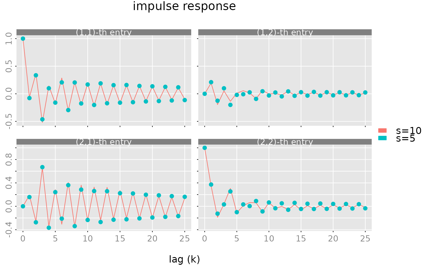
# example C (balanced truncation) ##########################

# construct a random rational matrix with statespace dimension s=10
obj = test_stsp(dim = c(2,2), s = 10, bpoles = 1, bzeroes = 1)
# compute an approximate realization with s0 = 8
gr = grammians(obj, 'minimum phase')
trunc = balance(obj, gr, s0 = 5)
print(trunc$sigma)
#>  [1] 4.93109117 1.21337534 0.98056829 0.55767576 0.48246007 0.26430938
#>  [7] 0.19433453 0.17190152 0.09269254 0.01001912

max(abs(unclass(pseries(obj, lag.max = 25)) - 
        unclass(pseries(trunc$ob, lag.max = 25))))
#> [1] 0.09578358
plot(pseries(obj, lag.max = 25), x_list= list(pseries(trunc$obj, lag.max = 25)), 
     type = c('l','p'), legend = c('s=10', 's=5'))