Plot Methods — plot methods • rationalmatrices

Plot impulse and frequency response functions.

Usage

# S3 method for pseries
plot(
  x,
  x_list = NULL,
  xlim = c("global", "column", "subfig"),
  ylim = c("row", "subfig", "global"),
  main = "impulse response",
  xlab = "lag (k)",
  ylab = NULL,
  subfigure_main = NA,
  parse_subfigure_main = FALSE,
  style = c("gray", "bw", "bw2", "colored"),
  col = NA,
  type = "l",
  lty = "solid",
  lwd = 1,
  pch = 16,
  cex.points = 1,
  bg.points = "black",
  legend = NULL,
  legend_args = NA,
  ...
)

# S3 method for zvalues
plot(
  x,
  x_list = NULL,
  style = c("gray", "bw", "colored"),
  which = c("modulus", "phase", "nyquist", "real"),
  subfigure_main = NA,
  xlim = NA,
  ylim = NA,
  main = NA,
  ylab = NA,
  xlab = NA,
  legend = NULL,
  legend_args = NA,
  col = NA,
  type = "l",
  lty = "solid",
  lwd = 1,
  pch = 16,
  cex.points = 1,
  bg.points = "black",
  ...
)

Arguments

x: pseries or zvalues object.
x_list: (optional) list of additional pseries or zvalues objects.
xlim, ylim: determine the axis limits of the subfigures. E.g. xlim = 'column' means that all subfigures in a column use the same x-axis limits. The parameter xlim may also contain a 2-dimensional vector c(x1,x2). In this case all sub-figures use the given limits for the x-axis. Furthermore the limits for the y-axis are computed based on the corresponding data "subset".
main: (character or expression) main title of the plot
xlab: (character string or expression) label for the x-axis
ylab: (character or expression) label for the y-axis
subfigure_main: scalar or (m x n) matrix of type "character" with the titles for the subfigures. If subfigure_main is a scalar character string then the procedures creates a matrix of respective titles by replacing the "place holders" 'i_' and 'j_' with the respective row and column number.
parse_subfigure_main: boolean. If TRUE then the titles for the subfigures are parsed to expression before plotting. See also plotmath on the usage of expressions for plot annotations.
style: (character string) determines the appearance of the plot (background color of the plot regions, color and line style of the grid lines, axis color, ...) See also style_parameters.
col: vector of line colors
type: vector of plot types. The following values are possible: "p" for points, "l" for lines, "b" for both points and lines, "c" for empty points joined by lines, "o" for overplotted points and lines, "s" and "S" for stair steps and "h" for histogram-like vertical lines. 'n' suppresses plotting.
lty: vector of line types. Line types can either be specified as integers (0=blank, 1=solid (default), 2=dashed, 3=dotted, 4=dotdash, 5=longdash, 6=twodash) or as one of the character strings "blank", "solid", "dashed", "dotted", "dotdash", "longdash", or "twodash", where "blank" uses ‘invisible lines’ (i.e., does not draw them).
lwd: vector of line widths.
pch: vector of plotting character or symbols. See points for possible values.
cex.points: vector of scales for the plotting symbols.
bg.points: vector of fill color for the open plot symbols.
legend: (character or expression vector). If NULL then no legend is produced.
legend_args: (optional) list with parameters for the legend. A legend title can be included with legend_args = list(title = my_legend_title). Note that the slots x, y are ignored and the legend is always put at the right hand side of the plot. See also legend.
...: not used.
which: (character string) what to plot (only used for zvalues objects). See details.

Value

The plot methods return (invisibly) a function, subfig say, which may be used to add additional graphic elements to the subfigures. The call opar = subfig(i,j)

creates a new (sub) plot at the (i,j)-the position with suitable margins and axis limits. See the examples below.

Details

The parameter which determines what to plot in the case of zvalues objects.

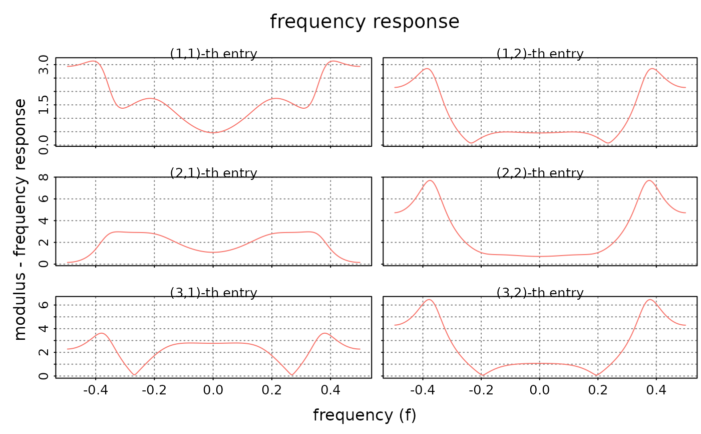
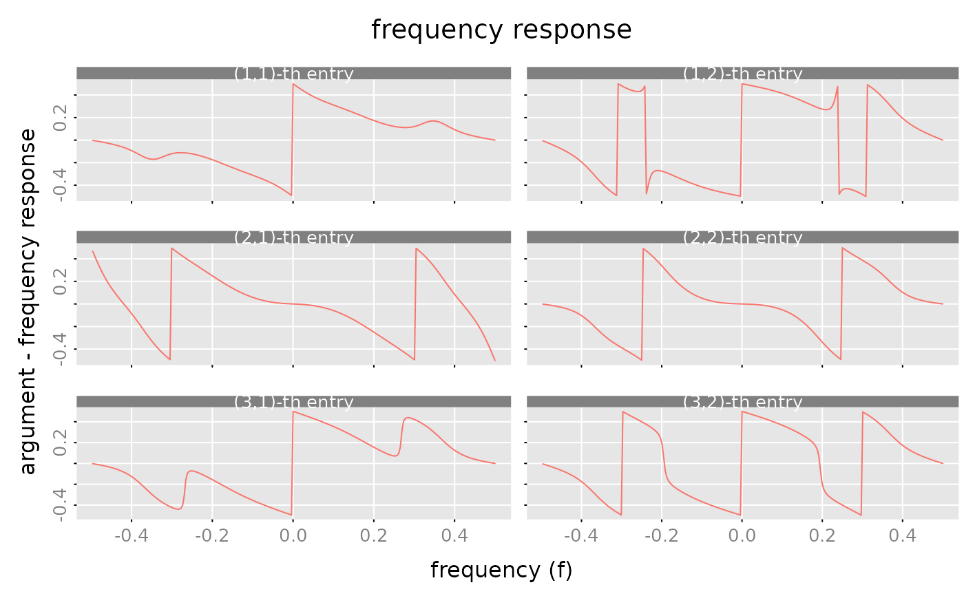
modulus: plot the moduli abs(x[i,j]) versus frequencies -Arg(z)/(2*pi).
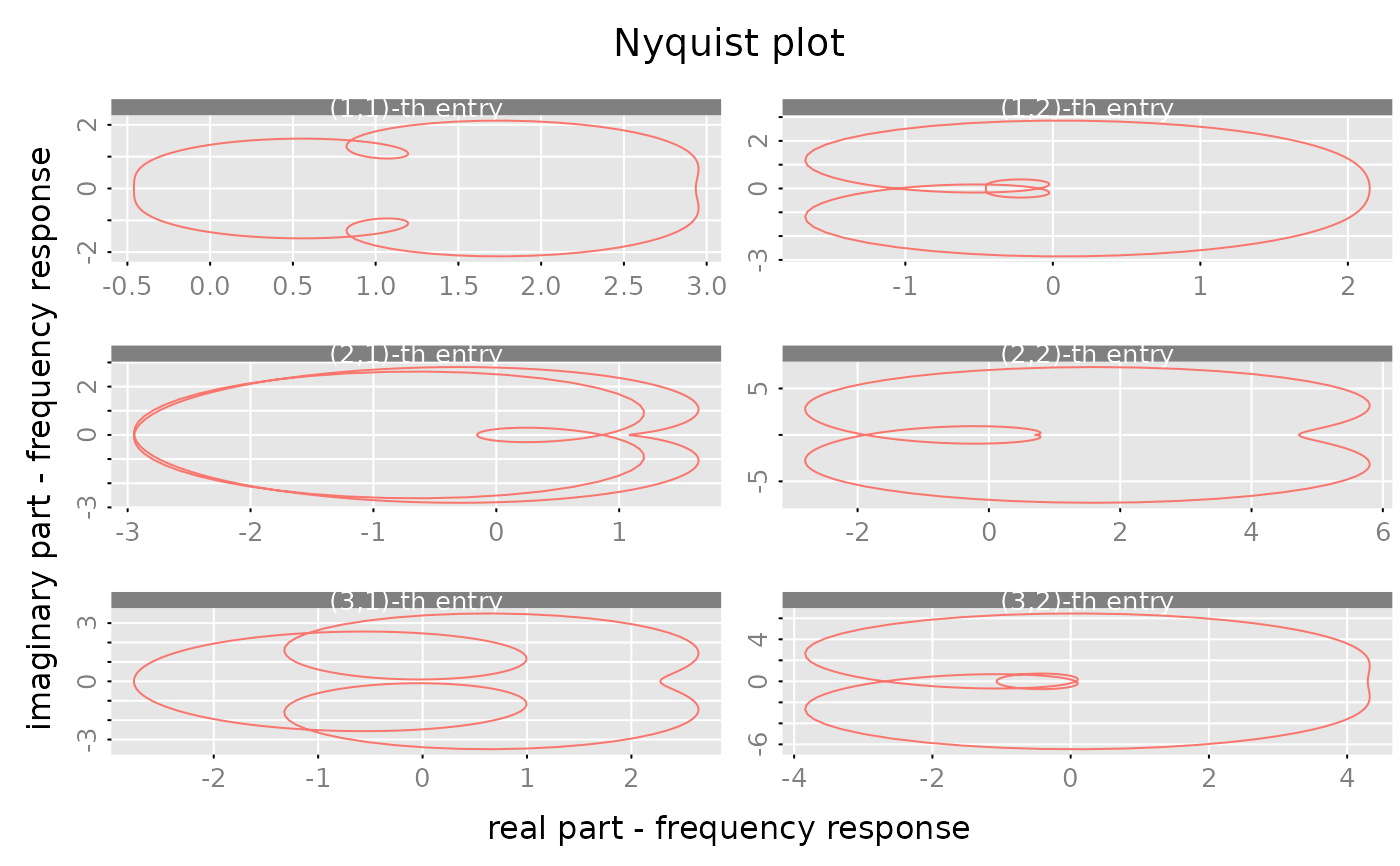
phase: plot the arguments Arg(x[i,j]) versus frequencies -Arg(z)/(2*pi).
nyquist: plot the imaginary part Im(x[i,j]) versus the real part Re(x[i,j]).
real: plot the real part Re(x[i,j]) versus the real part Re(z).

The choices which = 'modulus', which = 'phase' and which = 'nyquist' are typically used for the case, where the rational matrix is evaluated on a (regular) grid of points on the unit circle ($|z|=1$). The choice which = 'real' is of course designed for the case that the z's are real numbers.

NA values for the (optional) parameters mean that the methods use some suitable default values. (For the frequency response plots, e.g. the labels for the x- and y-axis are chosen according to the parameter which.)

NUll values for the (optional) parameters mean that the respective graphic element is omitted. E.g. subfigure_main=NULL skips the titles for the subfigures.

The titles for the (m,n) subfigures are determined by the parameter subfigure_main. One may pass an $(m,n)$ matrix of character strings to the procedure. Alternatively one may also provide an expression vector with a dim attribute such that subfigure_main[i,j] returns the expression which is to be used as title for the $(i,j)$-th subfigure. E.g. for a $(2,2)$ rational matrix one might use


subfigure_main = expression(Alpha, Beta, Gamma, Delta)
dim(subfigure_main) = c(2,2)

If subfigure_main is a scalar (character string or expression) then the procedures creates the respective titles by replacing the "place holders" i_ and j_ with the respective row and column number. See the examples below.

The parameter xlim determines the x-axis of the subfigures. If xlim='subfigure' then each subfigure gets its own x-axis (with different limits). For the case xlim='column' the subfigues in each column share a common x-axis (with common limits). The case xlim = 'global' means that all subfigures have the (x-) limits and the x-axis is only displayed for the subfigures in the last row. The parameter ylim is handled analogously.

If more than one object is plotted (if the optional parameter x_list is not empty) then a suitable legend may be added with the parameters legend, legend_args. Suppose that $k$ objects are plotted, then legend should be a character (or expression) vector of length k.

The "style" parameters col, type, ..., bg.points determine the appearance of the "lines" for each of the k objects. (If necessary the values are "recycled".)

These plot methods use the internal helper function plot_3D.

Examples

# Example for PSERIES ####################

# Generate a random, stable rational matrix a(z) in state space form (m = 3, n = 2, s = 4).
a = test_stsp(dim = c(3,2), s = 4, bpoles = 1)

# Generate a power series from this state space system
x = pseries(a, lag.max = 25)

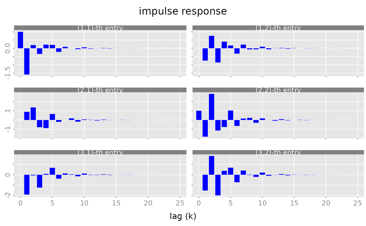
# create 'barplot'-like plot of the impulse response
#   the parameter 'lwd' has to be chosen accordingly
#   to the plot size and the number of lags!
par(lend = 'butt') # line end style: butt line caps
plot(x, type = 'h', lwd = 10, col = 'blue')


par(lend = 'round') # reset line end style to the default: rounded line caps


# Example for different plot types involving ZVALUES ####################

x = zvalues(a, n.f = 256)
plot(x, style = 'bw')

plot(x, which = 'phase')

plot(x, which = 'nyquist')



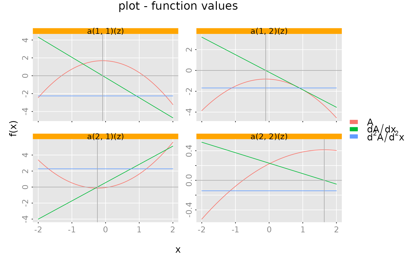
# Example for ZVALUES ####################

# Create a random polynomial  matrix (2,2)
a = test_polm(dim = c(2,2), degree = 2, random = TRUE)

# grid of x-values
x = seq(from = -2, to = 2, length.out = 101) 

subfig = plot(zvalues(a, z = x), 
              x_list = list(zvalues(derivative(a), z = x), 
                            zvalues(derivative(derivative(a)), z = x)), 
              style = 'colored', 
              which = 'real', 
              ylim = 'subfig', 
              legend = c(expression(A), expression(dA/dx), expression(d^2*A/d^2*x)), 
              subfigure_main = "a(i_, j_)(z)")
              
# Add horizontal/vertical lines       
opar = subfig(1,1)  # save graphic parameters
da = derivative(a)
for (i in (1:2)) {
   for (j in (1:2)) {
      subfig(i,j)
      graphics::abline(h = 0, col = 'darkgray')
      graphics::abline(v = polyroot(unclass(da[i,j])), col = 'darkgray')
}} 

graphics::par(opar)  # reset graphic parameters