Plot Forecast Error Variance Decomposition

Usage

# S3 method for fevardec
plot(
  x,
  main = NA,
  xlab = NA,
  col = NA,
  y_names = x$names,
  u_names = y_names,
  parse_names = FALSE,
  ...
)

Arguments

x: fevardec() object.
main: (character string) overall title for the plot. main=NULL omits the title and main = NA sets a default title.
xlab: (character string) title for the x-axis. xlab=NULL omits the title and xlab = NA sets a default x-axis title.
col: (m)-dimensional vector of colors. If NA then a default colormap is chosen.
y_names: optional (m)-dimensional character vector with names for the components of the time-series/process.
u_names: optional (m)-dimensional character vector with names for the orthogonalized shocks.
parse_names: boolean. If TRUE then the series- and shock- names are parsed to expression() before plotting. See also grDevices::plotmath() on the usage of expressions for plot annotations.
...: not used.

Value

This plot routine returns (invisibly) a function, subfig say, which may be used to add additional graphic elements to the subfigures. The call opar = subfig(i) creates a new (sub) plot at the (i)-th position with suitable margins and axis limits. See the example below.

Examples

# set seed for reproducible results
set.seed(1995)

model = test_stspmod(dim = c(2,2), s = 3, bpoles = 1, bzeroes = 1)
model$names = c('x[t]', 'y[t]')

# impulse response
irf = impresp(model, lag.max = 11, H = 'eigen')

# forecast error variance decomposition
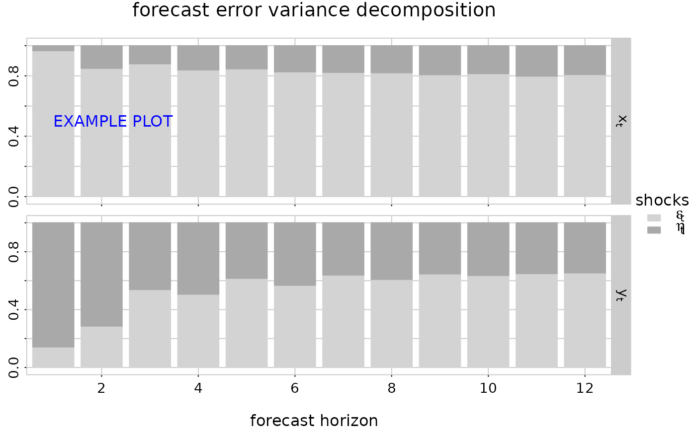
fevd = fevardec(irf)
# plot it
subfig = plot(fevd, col = c('lightgray','darkgray'),
              u_names = c('epsilon[t]', 'eta[t]'), parse_names = TRUE)

opar = subfig(1)
graphics::text(x = 1, y = 0.5, 'EXAMPLE PLOT', col = 'blue', adj = c(0, 0.5))

graphics::par(opar)

# reset seed
set.seed(NULL)