Case Study

Data

For this simple case study we use the Blanchard/Quah (1989) dataset with quarterly data of real GDP growth rates and the detrended unemployment rate in the USA.

y = BQdata_xts

break_date = as_date("1970-01-01")

y_train = BQdata_xts[index(BQdata_xts) < break_date]
y_test  = BQdata_xts[index(BQdata_xts) >= break_date]
dim_out = ncol(y_train)

plot(y)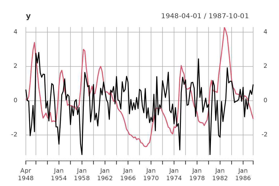

addLegend('topleft', c('GDP growth rate', 'Unemployment rate'), col = c('black', 'red'),
       lwd = 2, bty = 'n')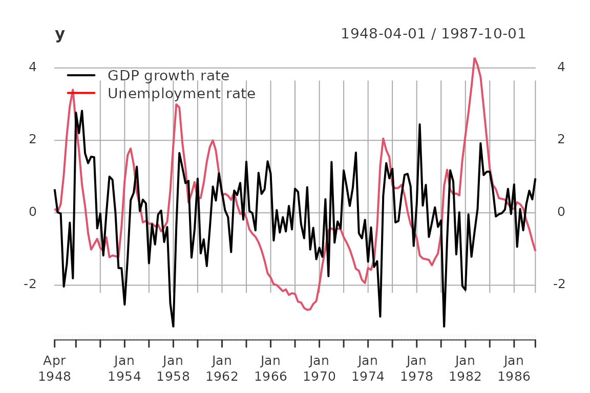

addEventLines(xts("Break", break_date))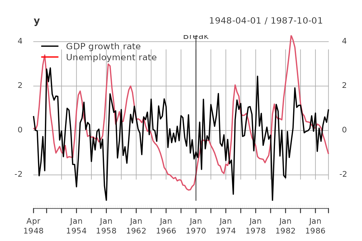

The data set contains 159 observations from 1948-04-01 to 1987-10-01. For estimation we use the first 87 observation till 1969-10-01.

The data is scaled such that the sample variances of the two series are equal to one.

AR Model

Here, we estimate an AR model where the order is determined via AIC. The only essential input for the function est_ar() is a data-object, e.g. a matrix with observations in rows and variables in columns, or a covariance-object. The defaults are using AIC for model selection, Yule-Walker estimation, and the sample.mean for estimating the \(\mathbb{E}\left(y_t\right)\).

out = est_ar(y_train, mean_estimate = 'zero')
out %>% names()
#> [1] "model"  "p"      "stats"  "y.mean" "ll"

Important statistics regarding model selection are contained in the slot stats

out$stats

p	n.par	lndetSigma	ic
0	0	1.013188	1.013188
1	4	-2.193313	-2.101359
2	8	-2.231092	-2.047184
3	12	-2.257910	-1.982047
4	16	-2.317073	-1.949257
5	20	-2.336830	-1.877060
6	24	-2.362950	-1.811226
7	28	-2.380498	-1.736819
8	32	-2.452787	-1.717155
9	36	-2.461676	-1.634090
10	40	-2.522346	-1.602806
11	44	-2.539423	-1.527929
12	48	-2.565177	-1.461728

The estimates as armamod object are stored in

out$model
#> ARMA model [2,2] with orders p = 1 and q = 0
#> AR polynomial a(z):
#>      z^0 [,1]  [,2]   z^1 [,1]       [,2]
#> [1,]        1     0 -0.4579266 -0.1795184
#> [2,]        0     1  0.3098179 -0.9328347
#> MA polynomial b(z):
#>      z^0 [,1]  [,2]
#> [1,]        1     0
#> [2,]        0     1
#> Left square root of noise covariance Sigma:
#>            u[1]      u[2]
#> u[1]  0.9567816 0.0000000
#> u[2] -0.2050479 0.3490723

The remaining slots are

out$ll
#> [1] -1.741221
out$p
#> [1] 1
out$y.mean
#> [1] 0 0

The estimated models are collected in two lists modelsand estimates.

models    = list(AR1 = out$model)
estimates = list(AR1 = list(model = out$model, n.par = out$p * dim_out^2))

Statespace Models

CCA Estimate

out = est_stsp_ss(y_train, method = 'cca', mean_estimate = 'zero')
out %>% names()
#> [1] "model"  "models" "s"      "stats"  "info"   "y.mean"

out$model
#> state space model [2,2] with s = 2 states
#>            s[1]       s[2]       u[1]      u[2]
#> s[1]  0.9191263  0.1912447 -0.1103757 0.7043585
#> s[2] -0.3340845  0.6472138 -0.6742802 0.2083379
#> x[1]  0.1800227 -0.5626354  1.0000000 0.0000000
#> x[2]  1.4254461  0.1339044  0.0000000 1.0000000
#> Left square root of noise covariance Sigma:
#>            u[1]      u[2]
#> u[1]  0.9477920 0.0000000
#> u[2] -0.1968541 0.3460504

Only the “chosen” model with s=1 has a value for lndetSigma below because the order selection criteria is performed first (and based on the singular values of the “normalized” Hankel matrix).

out$stats

s	n.par	Hsv	lndetSigma	criterion
0	0	NA	NA	0.9480826
1	4	0.9736953	NA	0.5022205
2	8	0.5448774	-2.229582	0.4863466
3	12	0.2751153	NA	0.6217772
4	16	0.0760915	NA	0.8213164

The slot models (plural) is only non-NULL if keep_models == TRUE.

out$models
#> NULL

Save the model

models$CCA    = out$model
estimates$CCA = list(model = out$model, n.par = 2*dim_out*out$s)

DDLC estimate

ML estimation of statespace model with a “DDLC” parametrization. We use the concentrated log likelihood, hence the noise covariance is not parametrized!

Of course, we should wrap this procedure into a suitable estimation procedure/function.

tmpl = tmpl_DDLC(models$CCA, balance = 'minimum phase', sigma_L = 'identity')
th0 = numeric(tmpl$n.par)

llfun = ll_FUN(tmpl, y_train, skip = 0, which = "concentrated")
control = list(trace = 1, fnscale = -1, maxit = 10)

out = optim(th0, llfun, method = 'BFGS', control = control)
#> initial  value 1.440187 
#> iter  10 value 1.393777
#> final  value 1.393777 
#> stopped after 10 iterations
th = out$par
model = fill_template(th, tmpl)

# reparametrize
tmpl = tmpl_DDLC(model, balance = 'minimum phase', sigma_L = 'identity')
llfun = ll_FUN(tmpl, y_train, skip = 0, which = "concentrated")
control$maxit = 20

out = optim(th0, llfun, method = 'BFGS', control = control)
#> initial  value 1.393777 
#> iter  10 value 1.393607
#> final  value 1.393607 
#> converged
th = out$par
model = fill_template(th, tmpl)

# reparametrize
tmpl = tmpl_DDLC(model, balance = 'minimum phase', sigma_L = 'identity')
llfun = ll_FUN(tmpl, y_train, skip = 0, which = "concentrated")
control$maxit = 200

out   = optim(th0, llfun, method = 'BFGS', control = control)
#> initial  value 1.393607 
#> final  value 1.393607 
#> converged
th    = out$par
model = fill_template(th, tmpl)

# out           = ll(model, y_train, skip = 0, which = "concentrated")
model$sigma_L = t(chol(model$sigma_L))

models$DDLC    = model
estimates$DDLC = list(model = model, n.par = tmpl$n.par)

ML Estimate of Echelon Form Model

ML estimation of the statespace model in echelon canonical form. We first have to coerce the CCA estimate into echelon canonical form.

lag.max = 20
ir = impresp(models$CCA, lag.max = lag.max)$irf # impulse response
nu = pseries2nu(ir)                             # Kronecker indices 
nu
#> [1] 1 1

# transform the CCA estimate into echelon canonical form
model = stspmod(sys = pseries2stsp(ir, method = 'echelon')$Xs, 
                sigma_L = models$CCA$sigma_L)
# check 
all.equal(autocov(model, lag.max = lag.max), 
          autocov(models$CCA, lag.max = lag.max))
#> [1] TRUE

tmpl = tmpl_stsp_echelon(nu, sigma_L = 'identity')
th0 = extract_theta(model, tmpl, on_error = 'stop', ignore_sigma_L = TRUE)

llfun = ll_FUN(tmpl, y_train, skip = 0, which = "concentrated")

control$maxit = 500 
out = optim(th0, llfun, method = 'BFGS', control = control)
#> initial  value 1.440187 
#> iter  10 value 1.393688
#> final  value 1.393607 
#> converged
th = out$par
model = fill_template(th, tmpl)
out = ll(model, y_train, skip = 0, which = "concentrated")
# model$sigma_L = t(chol(out$S))

models$SSECF    = model
estimates$SSECF = list(model = model, n.par = tmpl$n.par)

ARMA models

HRK estimate

Initial estimate via HRK procedure. This should be replaced with est_arma_hrk3().

tmpl = tmpl_arma_echelon(nu, sigma_L = 'chol')
out = est_arma_hrk(y_train, tmpl = tmpl, mean_estimate = 'zero')
#> HRK estimation of ARMA model: m=2, n.obs=87, p=1, q=1
#> initial AR estimate of noise p.max=9, p=8, ll=-1.085391
#> iter |th - th0|  n.val      MSE       ll 
#>    1      0.967     78    0.846   -1.282
models$HRK = out$model
estimates$HRK = list(model = out$model, n.par = tmpl$n.par - dim_out*(dim_out+1)/2)

ML Estimate of Echelon Form Model

ML estimation of ARMA model in echelon form.

tmpl = tmpl_arma_echelon(nu, sigma_L = 'identity')
th0 = extract_theta(models$HRK, tmpl, on_error = 'stop', ignore_sigma_L = TRUE)

llfun = ll_FUN(tmpl, y_train, skip = 0, which = "concentrated")

out = optim(th0, llfun, method = 'BFGS', control = control)
#> initial  value 1.404641 
#> iter  10 value 1.393736
#> final  value 1.393607 
#> converged
th = out$par
model = fill_template(th, tmpl)
out = ll(model, y_train, skip = 0, which = "concentrated")
# model$sigma_L = t(chol(out$S))

models$ARMAECF = model
estimates$ARMAECF = list(model = model, n.par = tmpl$n.par)

Compare Models

For this data set the three ML estimates are essentially equivalent:

all.equal(impresp(models$DDLC, lag.max = lag.max), 
          impresp(models$SSECF, lag.max = lag.max))
#> [1] "Component \"irf\": Mean relative difference: 2.075071e-05"
all.equal(impresp(models$DDLC, lag.max = lag.max), 
          impresp(models$ARMAECF, lag.max = lag.max))
#> [1] "Component \"irf\": Mean relative difference: 9.231668e-06"

Therefore we only keep the “SSECF” estimate for the further evluations/comparisons.

models = models[c('AR1','CCA','HRK','SSECF')]
estimates = estimates[c('AR1','CCA','HRK','SSECF')]

Portmanteau test for serial correlation for the AR1 estimate:

u = solve_inverse_de(models$AR1$sys, as.matrix(y_train))$u
pm_test(u, 8, dim_out^2)

lags	Q	df	p
2	11.22127	4	0.0241866
3	12.63544	8	0.1250236
4	16.29370	12	0.1781512
5	19.35190	16	0.2508379
6	20.69316	20	0.4153864
7	31.86943	24	0.1302638
8	33.88714	28	0.2046137

Compare estimates: collect statistics/tests into a matrix for easy comparison:

stats = compare_estimates(estimates, y_train, n.lags = 8)
if (requireNamespace("kableExtra", quietly = TRUE)) {
  stats %>%
    kable() %>%
    kableExtra::kable_styling(bootstrap_options = c("striped", "hover"))
} else {
  stats
}

	#par	ll	AIC	BIC	FPE	PM test
AR1	4	-1.462270	3.016495	3.129870	0.0700046	0.2046137
CCA	8	-1.440187	3.064283	3.291033	0.0734647	0.0770933
HRK	8	-1.404641	2.993191	3.219941	0.0684233	0.2380290
SSECF	8	-1.393607	2.971121	3.197872	0.0669297	0.3550802

ACF

plot(autocov(y, lag.max = lag.max), 
     lapply(models, FUN = autocov, lag.max = lag.max),
     legend = c('sample', names(models)),
     col = c('black', default_colmap(length(models))))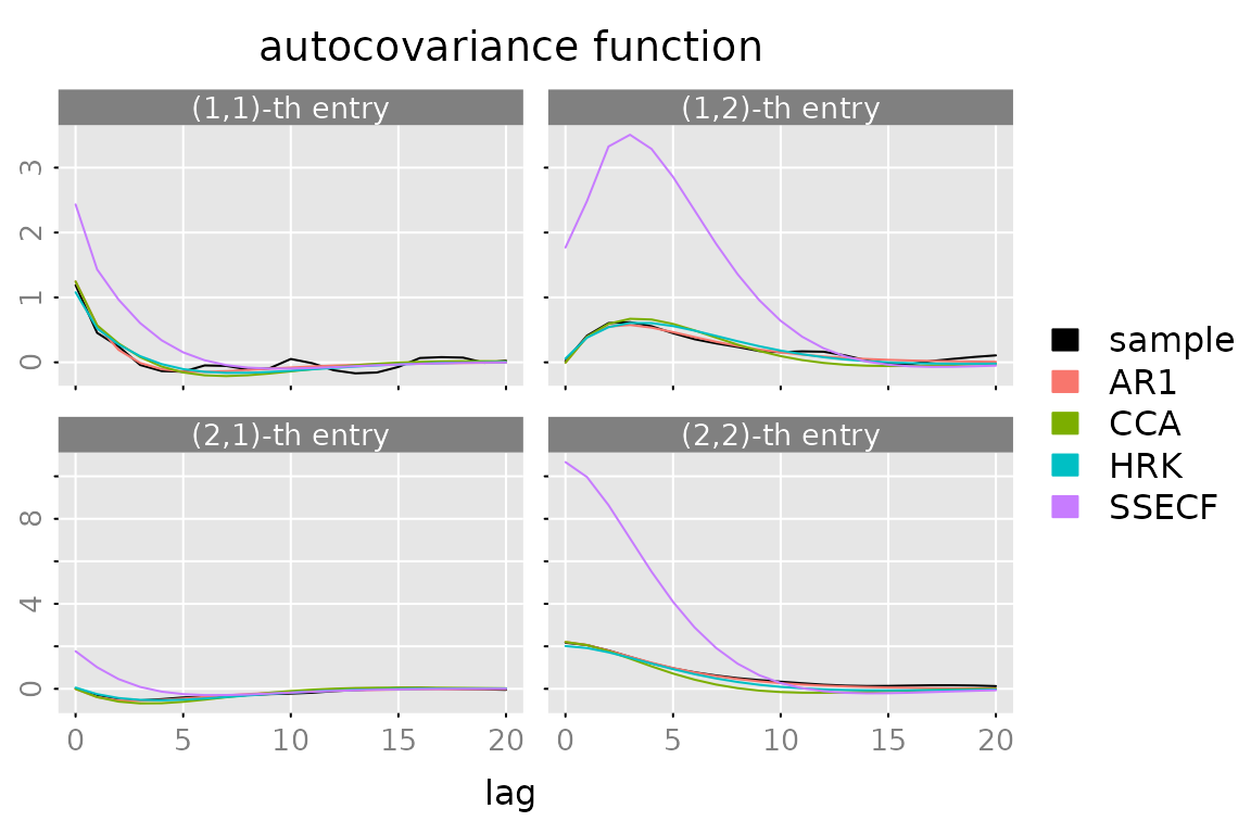

Spectral Density

plot(spectrald(models[[1]], n.f = 2^10), 
     lapply(models[-1], FUN = spectrald, n.f = 2^10),
     legend = names(models))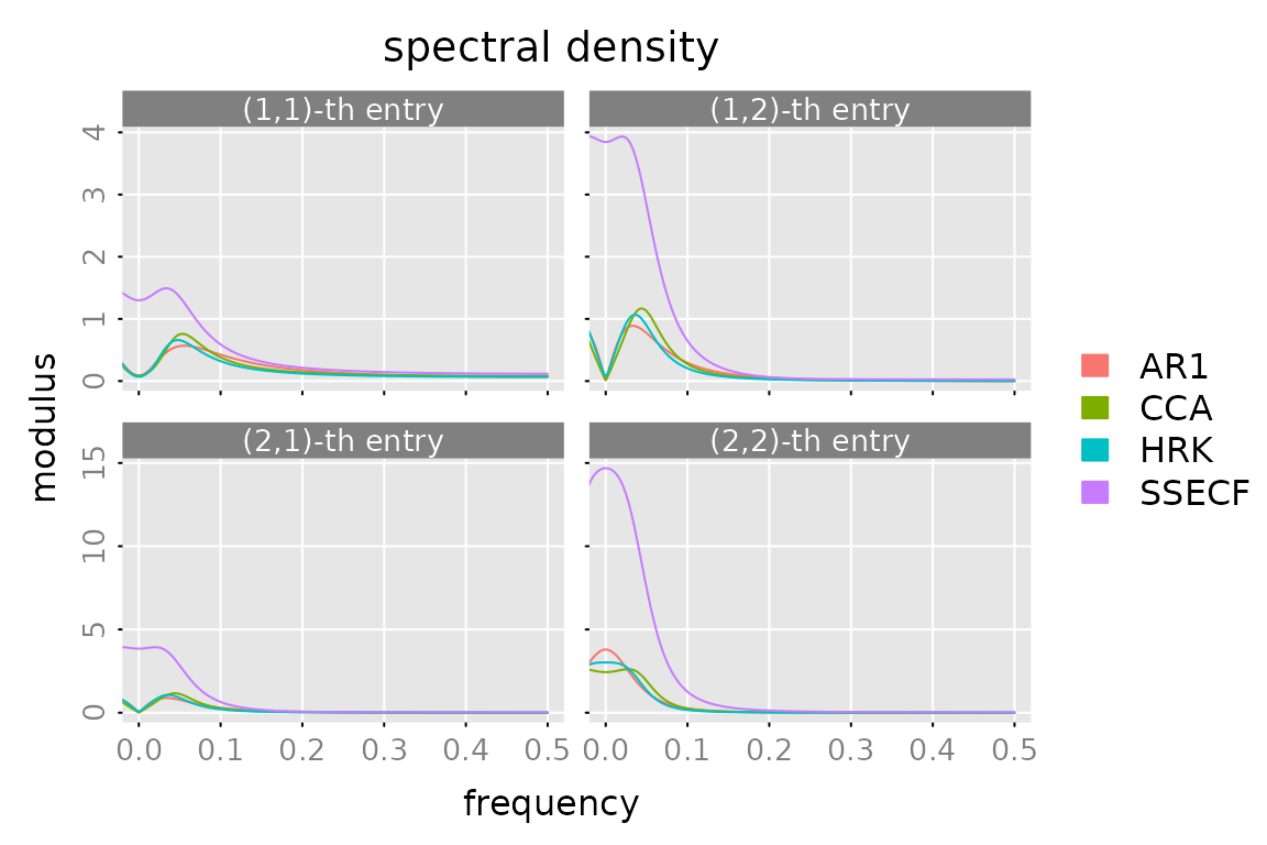

Impulse Response

plot(impresp(models[[1]], lag.max = lag.max), 
     lapply(models[-1], FUN = impresp, lag.max = lag.max),
     legend = names(models))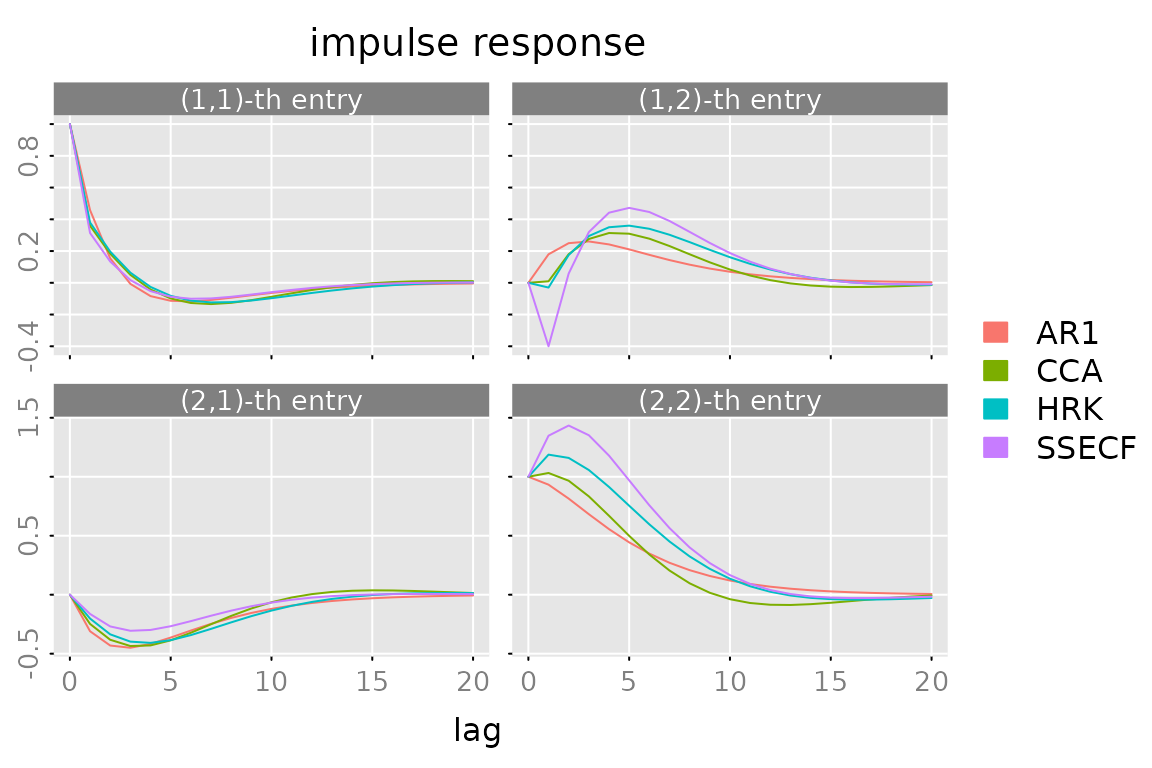

Prediction

Plot

n.ahead = 8
n.obs = nrow(y)
pred = predict(models$SSECF, y, h = c(1,4), n.ahead = n.ahead)
# add the date/time information to the list "pred"
# date = seq((start(y)-1)*3+1, by = 3, length.out = nrow(y)+n.ahead)
# date = as.Date(paste(start(y)[1] + (date-1) %/% 12, (date-1) %% 12 + 1, 1, sep='-'))
# pred$date = date

# the default "predictor names" h=1, h=2, ...
# don't look well, when plotted as expressions
dimnames(pred$yhat)[[3]] = gsub('=','==',dimnames(pred$yhat)[[3]])

# generate some plots ####################

# a simple/compressed plot of the data
p.y0 = plot_prediction(pred, which = 'y0', style = 'bw',
                       parse_names = TRUE, plot = FALSE)
p.y0()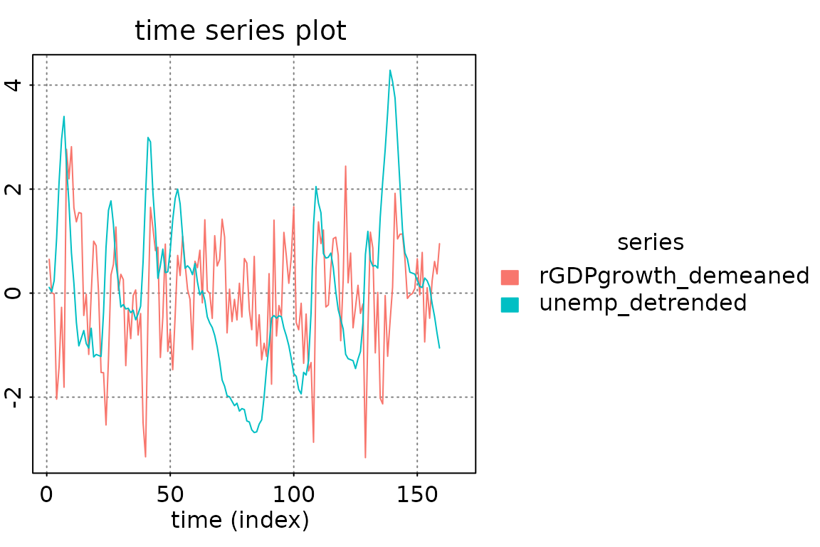


# a simple/compressed plot of the prediction errors
plot_prediction(pred, which = 'u0', parse_names = TRUE)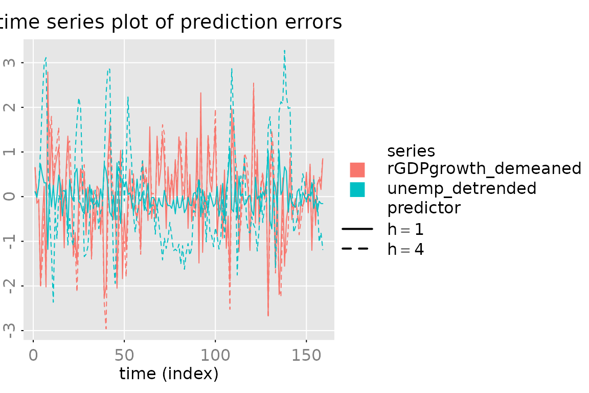


# plot of the prediction errors (with 95% confidence intervals)
plot_prediction(pred, which = 'error', qu = c(2,2,2),
                parse_names = TRUE)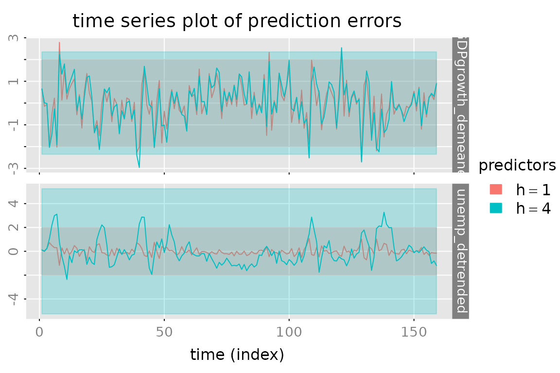


# plot of the true vales and the predicted values (+ 50% confidence region
# for the 1-step ahead prediction and the "out of sample" predictions)
p.y = plot_prediction(pred, qu = c(qnorm(0.75), NA, qnorm(0.75)),
                      parse_names = TRUE, plot = FALSE)
# subfig = p.y(xlim = date[c(n.obs-12, n.obs+n.ahead)])
# opar = subfig(1)
# abline(v = mean(as.numeric(date[c(n.obs, n.obs+1)])), col = 'red')
# # subfig(2)
# abline(v = mean(as.numeric(date[c(n.obs, n.obs+1)])), col = 'red')
# mtext(paste(' example plot:', date()), side = 1, outer = TRUE,
#       cex = 0.5, col = 'gray', adj = 0)
# graphics::par(opar) # reset the graphical parameters

# CUSUM plot of the prediction errors
plot_prediction(pred, which = 'cusum',
                style = 'gray', parse_names = TRUE)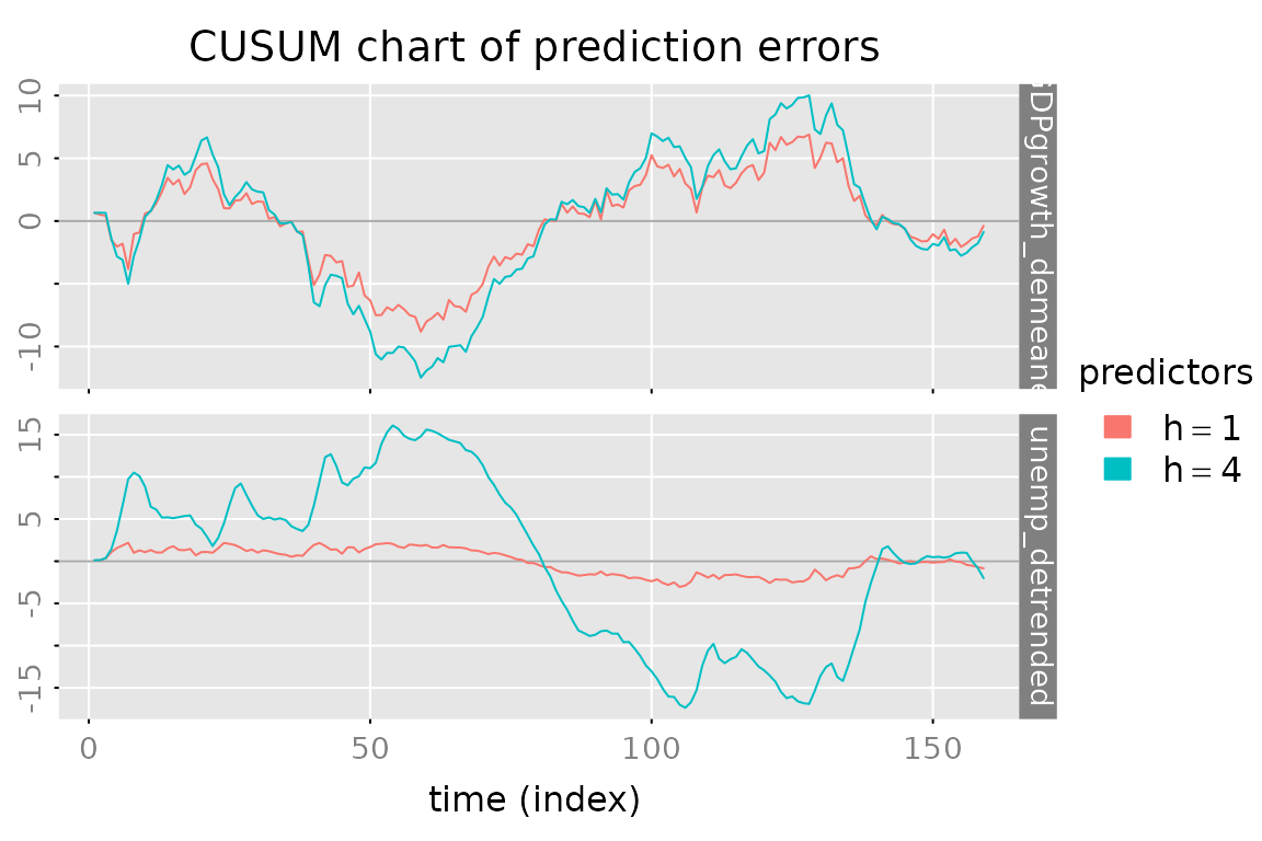


# CUSUM2 plot of the prediction errors
plot_prediction(pred, which = 'cusum2', parse_names = TRUE)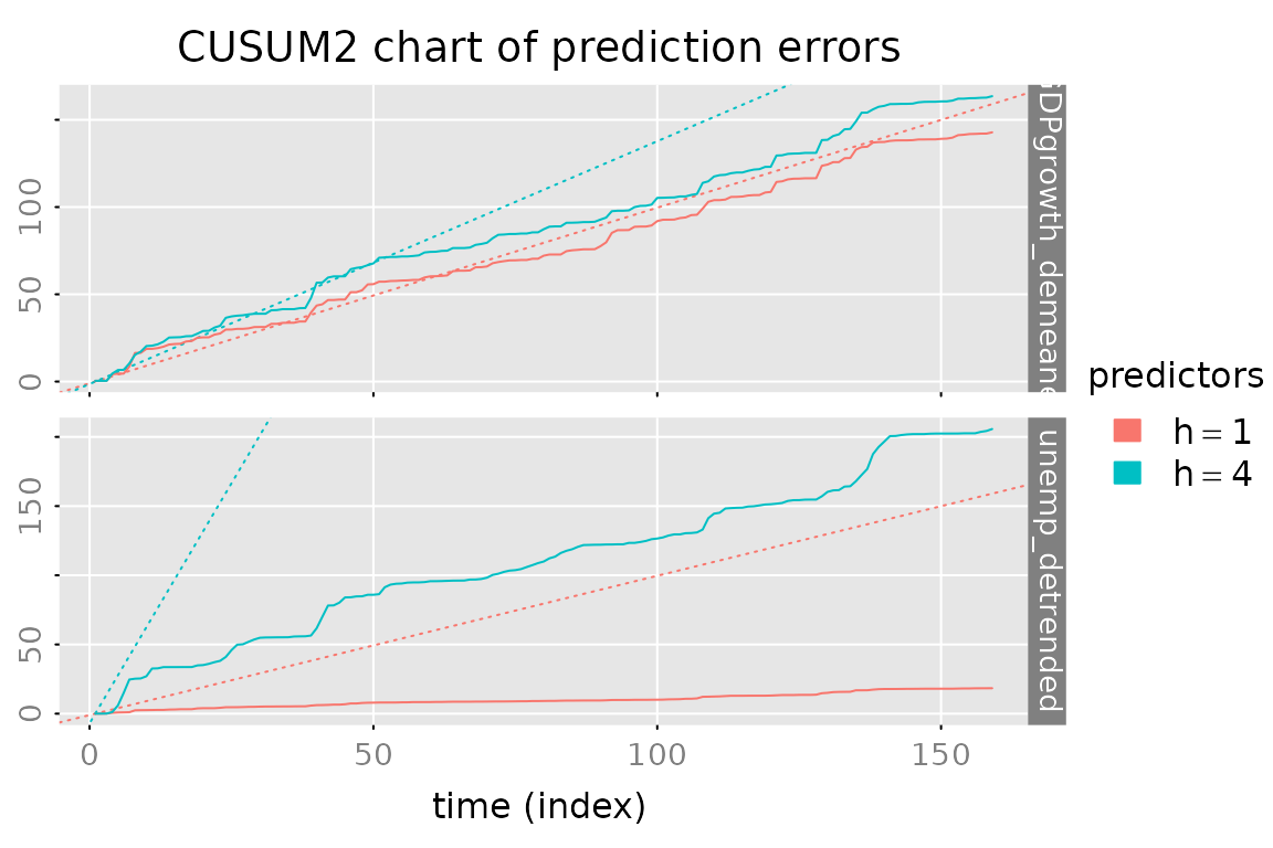

Evaluate and Compare Predictions

out = lapply(models, FUN = function(model) {predict(model, y, h = c(1,4))$yhat})
yhat = do.call(dbind, c(3, out) )
dimnames(yhat)[[3]] = kronecker(names(models), c(1,4), FUN = paste, sep = ':')
stats = evaluate_prediction(y, yhat, h = rep(c(1,4), length(models)), 
                            criteria = list('RMSE', 'MAE','MdAPE'), 
                            samples = list(in.sample = 1:dim(y_train), out.of.sample = (dim(y_train)+1):dim(y)))
#> Warning in 1:dim(y_train): numerical expression has 2 elements: only the first
#> used
#> Warning in (dim(y_train) + 1):dim(y): numerical expression has 2 elements: only
#> the first used
# dimnames.stats = dimnames(stats)
# stats = stats[,,c(seq(from = 1, by = 2, length.out = 6), 
#                   seq(from = 2, by = 2, length.out = 6)), ]
# dim(stats) = c(3,2,6,2,3)
# dimnames(stats) = list(criterion = dimnames.stats[[1]], sample = dimnames.stats[[2]], 
#                        predictor = names(models), h = paste('h=', c(1,4), sep = ''),
#                        data = dimnames.stats[[4]])

# use array2data.frame for "tabular" display of the results
stats.df = array2data.frame(stats, cols = 4)
stats.df$h = sub("^.*:","", as.character(stats.df$predictor))
stats.df$predictor = sub(":.$","", as.character(stats.df$predictor))
stats.df = stats.df[c('sample','h','criterion','predictor','rGDPgrowth_demeaned','unemp_detrended','total')]
stats.df = stats.df[order(stats.df$sample, stats.df$h, stats.df$criterion, stats.df$predictor),]
rownames(stats.df) = NULL
if (requireNamespace("kableExtra", quietly = TRUE)) {
  stats.df %>% 
    kable() %>%
    kableExtra::kable_styling(bootstrap_options = c("striped", "hover")) %>%
    kableExtra::collapse_rows(columns = 1:3, valign = "top")
} else {
  stats.df
}

sample	h	criterion	predictor	rGDPgrowth_demeaned	unemp_detrended	total
in.sample	1	RMSE	AR1	0.9504558	0.3513187	0.7165162
in.sample	1	RMSE	CCA	0.9427683	0.3437713	0.7095741
in.sample	1	RMSE	HRK	0.9407539	0.3346972	0.7060595
in.sample	1	RMSE	SSECF	0.9333399	0.3308350	0.7002054
in.sample	1	MAE	AR1	0.7294001	0.2740340	0.5017170
in.sample	1	MAE	CCA	0.7251022	0.2685577	0.4968299
in.sample	1	MAE	HRK	0.7235106	0.2551712	0.4893409
in.sample	1	MAE	SSECF	0.7088170	0.2542711	0.4815441
in.sample	1	MdAPE	AR1	87.2678257	20.0342420	52.8897843
in.sample	1	MdAPE	CCA	87.4154926	20.1617150	55.5970431
in.sample	1	MdAPE	HRK	87.1643611	25.0826798	51.6317436
in.sample	1	MdAPE	SSECF	84.9945947	22.8700095	51.2517523
in.sample	4	RMSE	AR1	1.0305227	1.1728519	1.1039834
in.sample	4	RMSE	CCA	1.0340753	1.2132320	1.1272186
in.sample	4	RMSE	HRK	1.0345632	1.2004940	1.1206040
in.sample	4	RMSE	SSECF	1.0248524	1.1834136	1.1069756
in.sample	4	MAE	AR1	0.7948530	0.9146552	0.8547541
in.sample	4	MAE	CCA	0.8019147	0.9588347	0.8803747
in.sample	4	MAE	HRK	0.8024096	0.9421335	0.8722715
in.sample	4	MAE	SSECF	0.7968589	0.9257861	0.8613225
in.sample	4	MdAPE	AR1	95.5494245	73.4116911	89.7586084
in.sample	4	MdAPE	CCA	96.4454672	71.0146064	89.3042399
in.sample	4	MdAPE	HRK	96.3023047	76.2988191	87.6635597
in.sample	4	MdAPE	SSECF	96.2978539	73.5616172	89.2922635
out.of.sample	1	RMSE	AR1	0.9998889	0.3927995	0.7596279
out.of.sample	1	RMSE	CCA	0.9793181	0.3660492	0.7392753
out.of.sample	1	RMSE	HRK	0.9809187	0.3552497	0.7377005
out.of.sample	1	RMSE	SSECF	0.9649344	0.3509004	0.7260267
out.of.sample	1	MAE	AR1	0.7679097	0.2834695	0.5256896
out.of.sample	1	MAE	CCA	0.7502218	0.2662833	0.5082526
out.of.sample	1	MAE	HRK	0.7506223	0.2613681	0.5059952
out.of.sample	1	MAE	SSECF	0.7369045	0.2606049	0.4987547
out.of.sample	1	MdAPE	AR1	98.3441782	22.7222538	58.2744063
out.of.sample	1	MdAPE	CCA	92.9245008	22.9246684	50.3690920
out.of.sample	1	MdAPE	HRK	90.6979145	21.4635151	49.2354982
out.of.sample	1	MdAPE	SSECF	93.4737624	21.8190844	49.4180249
out.of.sample	4	RMSE	AR1	0.9960909	1.0842018	1.0410789
out.of.sample	4	RMSE	CCA	0.9983745	1.0728332	1.0362728
out.of.sample	4	RMSE	HRK	0.9976987	1.0674377	1.0331568
out.of.sample	4	RMSE	SSECF	1.0011304	1.0791390	1.0408657
out.of.sample	4	MAE	AR1	0.7582807	0.8265544	0.7924176
out.of.sample	4	MAE	CCA	0.7646327	0.8196955	0.7921641
out.of.sample	4	MAE	HRK	0.7634857	0.8137818	0.7886337
out.of.sample	4	MAE	SSECF	0.7677140	0.8146076	0.7911608
out.of.sample	4	MdAPE	AR1	94.3096618	67.6228769	86.3295065
out.of.sample	4	MdAPE	CCA	97.5873129	69.7855043	85.5228705
out.of.sample	4	MdAPE	HRK	95.2805283	69.9050687	85.1506287
out.of.sample	4	MdAPE	SSECF	97.9900632	66.4893310	84.2382402


stats.df %>% names()
#> [1] "sample"              "h"                   "criterion"          
#> [4] "predictor"           "rGDPgrowth_demeaned" "unemp_detrended"    
#> [7] "total"

WS

4/15/2020

Data

AR Model

Statespace Models

CCA Estimate

DDLC estimate

ML Estimate of Echelon Form Model

ARMA models

HRK estimate

ML Estimate of Echelon Form Model

Compare Models

ACF

Spectral Density

Impulse Response

Prediction

Plot

Evaluate and Compare Predictions