Estimate State Space Models with Subspace Methods

Estimate (respectively construct) a state space model from a given sample or a given (sample) autocovariance function.

Usage

est_stsp_ss(
  obj,
  method = c("cca", "aoki"),
  s.max = NULL,
  p = NULL,
  p.ar.max = NULL,
  p.factor = 2,
  extend_acf = FALSE,
  sample2acf = TRUE,
  estorder = estorder_SVC,
  keep_models = FALSE,
  mean_estimate = c("sample.mean", "zero"),
  n.obs = NULL,
  ...
)

Arguments

obj: Either a "time series" object (i.e as.matrix(obj) returns an $(N,m)$-dimensional numeric matrix) or an autocov() object (with $L$ lags) which represents an (estimated) autocovariance function. The type of the autocov object is irrelevant since est_stsp_ss always uses the slot obj$gamma which contains the autocovariance function.
method: Character string giving the method used to fit the model.
s.max: (integer) maximum order of the state space model. If NULL a default value is chosen based on the sample size $N$, respectively based on the number of lags $L$ of the ACF.
p: (integer) number of block columns of the Hankel matrix (size of the "past"). If NULL then p is chosen by fitting a "long" AR model.
p.ar.max: (integer) maximum order of the "long" AR model. If NULL a default choice is made. This parameter is only needed in the case p=NULL.
p.factor: (integer) If p=NULL, then the number of block columns of the Hankel matrix is set to $p = p_f\hat{p}_{AIC}$ where $p_f$ is this parameter p.factor and $\hat{p}_{AIC}$ is the (AIC) estimate of the order of the "long" AR model. See also est_ar().
extend_acf: (boolean) If TRUE then the ACF is extended via an AR(p) model (MEST).
sample2acf: (boolean) If obj is a data object and sample2acf is TRUE, then first the sample autocovariance function is computed and then used for the actual computations.
estorder: function, used to select the order of the state space model.
keep_models: (boolean) should the function return a list with estimated system of order 0:s.max?
mean_estimate: Character string giving the method used to estimate the mean $\mu = E y_t$. Default is to use the sample mean. See the details below.
n.obs: Optional integer which gives the sample size $N$. This parameter is only used, when obj is an autocov() object. If n.obs=NULL then the slot obj$n.obs is used. Note that obj$n.obs=NULL or obj$n.obs=Inf refers to the case of a population autocovariance function, i.e. $N=\infty$. For a "time series" object the sample size is of course set to the number of observations, i.e. n.obs = nrow(as.matrix(obj)). The sample size $N$ controls the computation of the default (maximum) orders and the estimation of the order of the state space model.
...: additional parameters, passed on to the order estimation routine.

Value

list with slots

model: a stsp() object, which represents the estimated state space model.
models: either NULL (if !keep_models) or a list with the parameters of the estimated models with orders (s=0:s.max+1). This slot may e.g. be used to estimate the model order by some user defined model selection procedure.
s: (integer) the estimate of the model order.
info: list with information about the data and the design parameters of the estimation procedure.
stats: ((s.max+1)-by-5)-dimensional matrix with statistics of the (estimated) state space models.
y.mean: estimate of the mean $\mu$.

Details

The procedure implements three subspace algorithms for the estimation of state space models, the AOKI method, as described in (Aoki 1990) and the CCA and MEST algorithms (see e.g. (Dahlen and Scherrer 2004) ). All three algorithms center on the weighted Hankel matrix $$(R_f')^{-T} H_{fp} R_p^{-1}$$ where the block Hankel matrix $H_{fp}$ is the covariance between the "past" $(y_{t-1}',\cdots,y_{t-p}')'$ and the "future" $(y_{t}',\cdots,y_{t+f-1}')'$ and $R_f$ and $R_p$ are the cholesky factors of the covariance matrices of the "future" and the "past" respectively. The singular values of this weighted Hankel matrix are the canonical correlation coefficients between the past and the future. Note that the implementation here always sets $f = p+1$.

AOKIs method is a realization algorithm, i.e. it reconstructs the underlying state space model from the (population) autocovariance function. To this end a Riccati equation has to be solved, see riccati(). If an estimated ACF is fed into this algorithm one obtains an estimate for the state space model. However note that this may fail (in particular the Riccati equation may have no positive definite solution) if the estimate of the ACF is not positive definite, if the Hankel matrix is too small or if state dimension is not correct.

The CCA method estimates the state space model by first constructing an estimate of the states. Then the parameter matrices are estimated via simple LS regressions. This procedure does not give the "true" model, even in the case when the population ACF is used. However, the "distance" between the true model and the estimated model converges to zero, if the estimate of the ACF converges to the population ACF and the size $p$ of the Hankel matrix converges to infinity.

There are two implementations of the CCA method:

If obj is a "time series" object and sample2acf==FALSE then the helper function est_stsp_cca_sample() is called. This implementation of CCA operates directly on the supplied data.
If obj is an autocov() object or when obj is a "time series" object and sample2acf==TRUE then the helper function est_stsp_cca() is called. This implementation uses an (estimated) autocovariance function. For a time series object, first the sample autocovariance function is computed and then fed into the helper function.

The key idea of the MEST algorithm is to first estimate a "long" AR model, convert this AR model to a state space model and then to use a "balancing and truncation" method to obtain the final estimate of the state space model. This scheme may be obtained by calling est_stsp_ss with the option extend_acf=TRUE: This option instructs the procedure to first estimate an AR(p) model and then to use this model to "extend" the ACF, i.e. to compute the values of the ACF for lags $p+1,\ldots,2p$. Then this extended ACF is fed into the helper function est_stsp_cca().

Note that MEST uses the autocovariance function. So for a "time series" object one has to set sample2acf=TRUE.

These algorithms may be used for model reduction (i.e. to find a model with a smaller state space dimension than the true model) and for estimation (by feeding a sample autocovariance function in).

These algorithms may also be used as simple "model reduction algorithms". If we want to approximate a high dimensional state space model by a model of lower order, we may proceed as follows. First we compute the ACF of the high dimensional model and then fed this ACF into the subspace routine est_stsp_ss, however setting the maximum order s.max to some value less than the true order. Note thet the AOKI procedure however, may break down, since it is not guaranteed that the Riccati equation, which needs to be solved, has a positive semidefinite solution.

Size of the Hankel matrix

If the input parameter p=NULL then $p$ is chosen as follows. The procedure estimates the order of a "long" AR model with the AIC criterion. The size of the "past" $p$ then is set to $p = p_f\hat{p}_{AIC}$ where $p_f$ is a factor (defaults to $2$) and $\hat{p}_{AIC}$ is the (AIC) estimate of the order of the "long" AR model. See also est_ar().

Estimation of the Mean

If the input parameter obj is an autocov() object (which contains no info about the mean $\mu=E y_t$) the "estimate" of the mean is simply set to a vector of NA's.

If the input parameter obj is a "time series" object, then there are two options. For mean_estimate == 'zero' the procedure assumes that the process is centered ($\mu=E y_t=0$) and thus sets the estimate to a zero vector. In the case mean_estimate == 'sample.mean' the sample mean of the data is used.

Order Estimation

The input parameter s.max defines the maximum order considered.

The order estimation is based on the Hankel singular values $\sigma_s$ and/or the log det values of the estimated noise covariance matrices $\ln\det \hat{\Sigma}_s$. Using only the Hankel singular values has the advantage that only one model has to be estimated, whereas otherwise estimates for all models with orders $s=0,\ldots,s_{\max}$ have to be computed.

In order to exploit this (small) advantage of singular values based criteria the order estimation runs as follows: First the procedures call
estorder(s.max, Hsv, n.par, m, n.obs, Hsize=c(f,p), ...)
Here Hsv is an $pm$ dimensional vector with the Hankel singular values and n.par is an $(s_{\max}+1)$ dimensional vector with the respective number of parameters of the models with orders $s=0,\ldots,s_{\max}$. If this call returns an estimate of the order then the procedures estimate a corresonding state space model.

If this call fails (i.e returns NULL) then the procedures estimate all models with orders up to $s_{\max}$ and the corresponding noise covariance matrices. The order then is estimated by calling
estorder(s.max = s.max, Hsv, lndetSigma, n.par, m, n.obs, Hsize, ...)
where lndetSigma is the vector with the log det values of the estimated noise covariance matrices ($\ln\det \hat{\Sigma}_s$).

The package offers some predefined order selection procedures (see also subspace order estimates):

estorder_max(s.max, ...) simply returns the maximum order s.max considered.
estorder_rkH(s.max, Hsv, tol, ...) estimates the order by an estimate of the rank of the Hankel matrix.
estorder_MOE(s.max, Hsv, ...) estimates the order by searching for a "gap" in the singular values.
estorder_SVC(s.max, Hsv, n.par, n.obs, Hsize, penalty, ...) implements the so called Singular Value Criteria, see (Bauer 2001) : $$svc(s) = \sigma_{s+1}^2 + c(N)d(s)/N$$ Here $\sigma_s$ is the $s$-th singular value of the weighted Hankel marix, $N$ is the sample size, $d(s) = 2ms$ denotes the number of parameters for a state space model with $s$ states (and $m$ outputs) and $c(N)$) is a "penalty" (depending on the sample size).
The above order estimation procedures only use the Hankel singular values, whereas the following procedure is based on the estimated noise covariances.
estorder_IVC(s.max, lndetSigma, n.par, n.obs, penalty, ...) estimates the order via an information criterion of the form $$ivc(s) = \ln\det\hat\Sigma_{s} + c(N)d(s)/N$$ where $\hat\Sigma_s$ is the estimate of the noise covariace matrix obtained from a model with order $s$, $d(s)$ denotes the number of parameters and $c(N)$ is a "penalty" (depending on the sample size).

For both estorder_SVC and estorder_IVC the (optional) parameter penalty controls the penalty term $c(N)$.

Further Notes

The actual computations are done by the helper routines detailed in subspace helpers.

The type of the autocov() object is irrelevenat since the function always uses the slot obj$gamma.

For keep_models==TRUE the estimation procedure compute all models even in the case of a Hankel singular value based selection criterion.

References

Aoki M (1990). State Space Modeling of Time Series. Springer Verlag, New York.

Bauer D (2001). “Order estimation for subspace methods.” Automatica, 37(10), 1561 - 1573. doi:10.1016/S0005-1098(01)00118-2 .

Dahlen A, Scherrer W (2004). “The relation of the CCA subspace method to a balanced reduction of an autoregressive model.” Journal of Econometrics, 118, 293--312. doi:10.1016/S0304-4076(03)00144-1 .

Examples

set.seed(3421) # in order to get reproducible results

# create a "random", stable and miniphase state space model
m = 2 # number of outputs
s = 3 # number of states
s.max = 2*s
lag.max = max(4*s, 25)
n.obs = 1000

model = r_model(tmpl_stsp_full(m, m, s),
                bpoles = 1, bzeroes = 1,  sd = 0.5)
# scale sigma_L
diag(model$sigma_L) = 1

# compute ACF
gam = autocov(model, lag.max = lag.max)

# simulate data
data = sim(model, n.obs)

# sample ACF
gam.sample = autocov(data$y, lag.max = lag.max, demean = FALSE)

# AOKIs method ##############################################################
# reconstruct the true model from the population ACF
# "estimate" the order by the rank of the Hankel matrix
out = est_stsp_ss(gam, method = 'aoki', s.max = 2*s, estorder = estorder_rkH)

# compute the ACF of the constructed model.
gam.hat = autocov(out$model, lag.max = lag.max)

# check that the constructed model is equivalent to the original model
all.equal(dim(model$sys), dim(out$model$sys))
#> [1] TRUE
all.equal(gam, gam.hat)
#> [1] TRUE


# CCA based on the sample ###################################################
# estimate the order by a "singular value criterion"
out = est_stsp_ss(data$y, method = 'cca', sample2acf = FALSE, s.max = 2*s,
                  estorder = estorder_SVC)

# compute the ACF of the constructed model.
gam.hat = autocov(out$model, lag.max = lag.max)

all.equal(dim(model$sys), dim(out$model$sys)) # the estimated order is correct
#> [1] TRUE
all.equal(gam$gamma, gam.hat$gamma)           # but of course the estimated model is not perfect
#> [1] "Mean relative difference: 0.1680467"

# CCA based on the sample ACF ###############################################
# estimate the order by an "information criterion"
out = est_stsp_ss(gam.sample, method = 'cca', s.max = 2*s,
                  estorder = estorder_IVC)

# compute the ACF of the constructed model.
gam.hat = autocov(out$model, lag.max = lag.max)

cat('s.hat=', dim(out$model$sys)[3], '\n') # the estimated order is s.hat=2, the true order is s=3!
#> s.hat= 2 
all.equal(gam$gamma, gam.hat$gamma)        # relative error of the TRUE and the estimated ACF
#> [1] "Mean relative difference: 0.1966654"

# alternatively, we may also use
out2 = est_stsp_ss(data$y, sample2acf = TRUE, mean_estimate = 'zero',
                   method = 'cca', s.max = 2*s, estorder = estorder_IVC)
all.equal(out$model, out2$model)
#> [1] TRUE

# MEST algorithm #############################################################
# estimate the order by an "information criterion"
out = est_stsp_ss(gam.sample, method = 'cca', extend_acf = TRUE, s.max = 2*s,
                  estorder = estorder_IVC)

# compute the ACF of the constructed model.
gam.hat = autocov(out$model, lag.max = lag.max)

cat('s.hat=', dim(out$model$sys)[3], '\n') # the estimated order is s.hat=2, the true order is s=3!
#> s.hat= 2 
all.equal(gam$gamma, gam.hat$gamma)        # relative error of the TRUE and the estimated ACF
#> [1] "Mean relative difference: 0.196599"

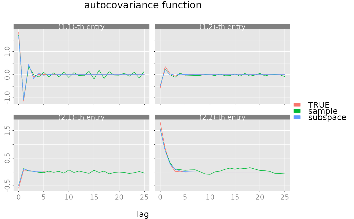
# make a plot of the ACFs
plot(gam, list(gam.sample, gam.hat), legend = c('TRUE', 'sample', 'subspace'))


# reset seed
set.seed(NULL)