Sequential Monte Carlo (Particle Filter) Methods

Implementation of Sequential Monte Carlo (SMC) methods, also known as particle filters, for state space models. These methods extend Kalman filtering to nonlinear and/or non-Gaussian state space models.

Usage

pfilter(
  model,
  y,
  method = c("sir", "apf", "optimal"),
  N_particles = 1000,
  resampling = c("systematic", "multinomial", "stratified"),
  ess_threshold = 0.5,
  P1 = NULL,
  a1 = NULL,
  ...
)

# S3 method for class 'stspmod'
pfilter(
  model,
  y,
  method = c("sir", "apf", "optimal"),
  N_particles = 1000,
  resampling = c("systematic", "multinomial", "stratified"),
  ess_threshold = 0.5,
  P1 = NULL,
  a1 = NULL,
  ...
)

Arguments

model: stspmod() object, which represents the state space model. For nonlinear models, additional parameters may be required.
y: sample, i.e. an $(N,m)$ dimensional matrix, or a "time series" object (i.e. as.matrix(y) should return an $(N,m)$-dimensional numeric matrix). Missing values (NA, NaN and Inf) are not supported.
method: Character string specifying the particle filter algorithm. Options: "sir" (Sampling Importance Resampling, default), "apf" (Auxiliary Particle Filter), "optimal" (Optimal proposal for linear Gaussian). Note: The APF method may produce biased likelihood estimates for models with cross-covariance between state and observation noise (S != 0). For linear Gaussian models with cross-correlation, the optimal proposal is recommended.
N_particles: Number of particles to use (default: 1000).
resampling: Resampling method: "multinomial", "systematic" (default), or "stratified".
ess_threshold: Effective sample size threshold for triggering resampling (default: 0.5). Resampling occurs when ESS < ess_threshold * N_particles.
P1: $(s,s)$ dimensional covariance matrix of the error of the initial state estimate, i.e. $\Pi_{1|0}$. If NULL, then the state covariance $P = APA'+B\Sigma B'$ is used.
a1: $s$ dimensional vector, which holds the initial estimate $a_{1|0}$ for the state at time $t=1$. If a1=NULL, then a zero vector is used.
...: Additional arguments passed to filter implementations.

Value

List with components

filtered_states: $(N+1,s)$ dimensional matrix with the filtered state estimates. The $t$-th row corresponds to $E[x_t | y_{1:t}]$.
predicted_states: $(N+1,s)$ dimensional matrix with the predicted state estimates. The $t$-th row corresponds to $E[x_t | y_{1:t-1}]$.
particles: $(s, N\_particles, N+1)$ dimensional array containing the particle trajectories.
weight_trajectories: $(N+1, N\_particles)$ dimensional matrix of particle weights over time. The $t$-th row corresponds to weights at time $t$.
weights: $(N\_particles)$ dimensional vector of normalized particle weights at final time.
log_likelihood: Particle approximation of the log-likelihood.
log_likelihood_contributions: $(N)$ dimensional vector of log-likelihood contributions per time step.
effective_sample_size: $(N+1)$ dimensional vector of effective sample sizes.
N_particles: Number of particles used.
resampling_method: Resampling method used.
filter_type: Type of particle filter used.

Details

The particle filter approximates the filtering distribution $p(x_t | y_{1:t})$ using a set of weighted particles (samples). The basic algorithm is the Sampling Importance Resampling (SIR) filter, also known as the bootstrap filter.

The model considered is $$x_{t+1} = f(x_t, u_t)$$ $$y_t = h(x_t, v_t)$$ where $f$ is the state transition function, $h$ is the observation function, and $u_t$, $v_t$ are noise processes.

For linear Gaussian models (the default), these reduce to $$x_{t+1} = A x_t + B u_t$$ $$y_t = C x_t + D v_t$$ with $u_t \sim N(0, Q)$ and $v_t \sim N(0, R)$.

Examples

# Linear Gaussian example: compare particle filter with Kalman filter
set.seed(123)
s = 2  # state dimension
m = 1  # number of outputs
n = m  # number of inputs
n.obs = 100 # sample size

# Generate a stable state space model
tmpl = tmpl_stsp_full(m, n, s, sigma_L = "chol")
model = r_model(tmpl, bpoles = 1, sd = 0.5)
# Generate a sample
data = sim(model, n.obs = n.obs, a1 = NA)

# Run particle filter
pf_result = pfilter(model, data$y, N_particles = 500)

# Compare with Kalman filter
kf_result = kf(model, data$y)

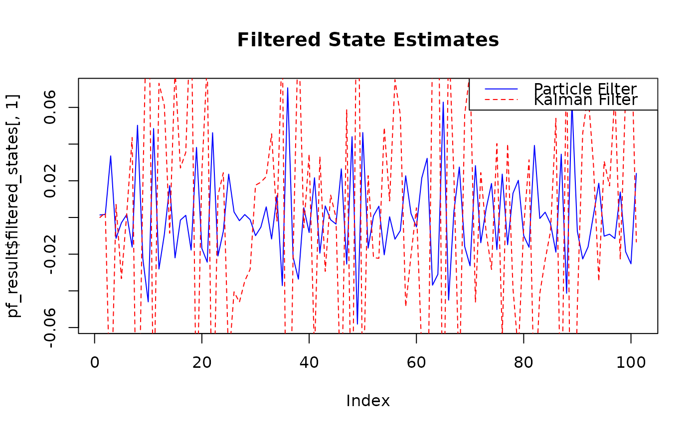
# Plot filtered states comparison
plot(pf_result$filtered_states[,1], type = "l", col = "blue",
     main = "Filtered State Estimates")
lines(kf_result$a[,1], col = "red", lty = 2)
legend("topright", legend = c("Particle Filter", "Kalman Filter"),
       col = c("blue", "red"), lty = 1:2)