Technical Reference: RLDM Classes and Methods

Wolfgang Scherrer and Bernd Funovits

2026-01-18

This document is a reference guide for RLDM classes, mathematical foundations, and estimation methods. For practical examples, see the “Getting Started” and “Case Study” vignettes.

---

Preliminaries

Notation

The following notation is used throughout RLDM:

Symbol	Meaning
$m$	Dimension of the output process $(y_t)$
$n$	Dimension of the noise process $(u_t)$, typically $n=m$
$s$	Dimension of the state process $(a_t)$ (state space models only)
$N$	Sample size, denoted n.obs in code
$\mathbb{E}$	Expectation operator
$\gamma_k$	Autocovariance at lag $k$
$\Sigma$	Noise covariance matrix $\mathbb{E}(u_t u_t')$

Sign Convention

RLDM uses a non-standard sign convention for AR coefficients to maintain consistency with matrix fraction descriptions.

Standard form (often seen in time series textbooks): $$y_t = a_1 y_{t-1} + a_2 y_{t-2} + \cdots + a_p y_{t-p} + u_t$$

RLDM form (matrix fraction description): $$y_t + a_1 y_{t-1} + a_2 y_{t-2} + \cdots + a_p y_{t-p} = u_t$$

Notice the opposite signs on the AR coefficients. This ensures consistency when working with rational matrix fractions where: $$a_0 y_t + a_1 y_{t-1} + \cdots + a_p y_{t-p} = b_0 u_t + b_1 u_{t-1} + \cdots + b_q u_{t-q}$$

with $a_0 = I_m$ (identity matrix).

---

Model Classes

Overview: Model Representations

RLDM supports three equivalent ways to represent rational linear dynamic models:

1. Left Matrix Fraction Description (LMFD): armamod

The ARMA/VARMA representation: $$a(z) y_t = b(z) u_t$$

where $a(z)$ and $b(z)$ are polynomial matrices in the lag operator $z$.

2. State Space Form: stspmod

The canonical state space representation: $$\begin{aligned} s_{t+1} &= A s_t + B u_t \\ y_t &= C s_t + D u_t \end{aligned}$$

where $s_t$ is the state vector of dimension $s$.

3. Right Matrix Fraction Description (RMFD): rmfdmod

An alternative ARMA representation (experimental): $$\begin{aligned} w_t &= c(z) u_{t} \\ y_t &= d(z) w_t \end{aligned}$$

---

VARMA/ARMA Models: armamod Class

The armamod class represents VARMA (multivariate ARMA) processes in left matrix fraction form.

Structure

An armamod object is an S3 list with the following slots:

Slot	Type	Description
sys	lmfd [m,n]	Left matrix fraction: filter $k(z) = a(z)^{-1}b(z)$
sigma_L	double [n,n]	Left square root of noise covariance ($\Sigma = LL'$)
names	character [m]	Component names of $y_t$
label	character	Descriptive label for the process

Class attribute: c("armamod", "rldm")

Constructor

armamod(sys, sigma_L, names = NULL, label = NULL)

Example:

# Create a simple AR(1) model: y_t = 0.8*y_{t-1} + u_t
# In RLDM convention: y_t - 0.8*y_{t-1} = u_t
a_coef <- matrix(-0.8)  # negative sign for standard convention
b_coef <- matrix(1)
sys <- lmfd(a_coef, b_coef)

model <- armamod(sys, sigma_L = matrix(1), names = "Output", label = "AR(1)")
model
#> AR(1): ARMA model [1,1] with orders p = 0 and q = 0
#> AR polynomial a(z):
#>      z^0 [,1]
#> [1,]     -0.8
#> MA polynomial b(z):
#>      z^0 [,1]
#> [1,]        1
#> Left square root of noise covariance Sigma:
#>      u[1]
#> u[1]    1

Available Methods

methods(class = 'armamod')
#>  [1] as.stspmod autocov    freqresp   impresp    ll         poles     
#>  [7] predict    print      sim        spectrald  str        zeroes    
#> see '?methods' for accessing help and source code

Key methods: - autocov() - Compute autocovariance function - impresp() - Impulse response functions - spectrald() - Spectral density - freqresp() - Frequency response - predict() - Forecasting - solve_de() - Simulate from the model - print() / plot() - Visualization

---

State Space Models: stspmod Class

The stspmod class represents processes in canonical state space form.

Structure

An stspmod object is an S3 list with slots:

Slot	Type	Description
sys	stsp [m,n]	State space realization
sigma_L	double [n,n]	Left factor of noise covariance
names	character [m]	Component names
label	character	Descriptive label

Class attribute: c("stspmod", "rldm")

Constructor

stspmod(sys, sigma_L, names = NULL, label = NULL)

Example:

# Create a simple state space model
# s_{t+1} = 0.8*s_t + u_t
# y_t = s_t

A_matrix <- matrix(0.8)
B_matrix <- matrix(1)
C_matrix <- matrix(1)
D_matrix <- matrix(0)

sys <- stsp(A_matrix, B_matrix, C_matrix, D_matrix)
model_ss <- stspmod(sys, sigma_L = matrix(1))
model_ss
#> state space model [1,1] with s = 1 states
#>      s[1] u[1]
#> s[1]  0.8    1
#> x[1]  1.0    0
#> Left square root of noise covariance Sigma:
#>      u[1]
#> u[1]    1

Available Methods

methods(class = 'stspmod')
#>  [1] autocov   freqresp  impresp   ll        poles     predict   print    
#>  [8] sim       spectrald str       zeroes   
#> see '?methods' for accessing help and source code

Similar to armamod, state space models support: - Autocovariance, impulse responses, spectral density computation - Forecasting and simulation - Conversion to impulse response representation

State Space Parameterizations

RLDM supports several standard state space canonical forms through template functions:

• tmpl_DDLC() - Diagonal-Direct-Lead-Coefficient form
• tmpl_stsp_echelon() - Echelon canonical form
• tmpl_stsp_innovation() - Innovation form

---

Right Matrix Fraction Description: rmfdmod Class

The rmfdmod class represents processes in right matrix fraction form (experimental, limited methods):

rmfdmod(sys, sigma_L, names = NULL, label = NULL)

Most estimation and analysis methods are not yet implemented for this class.

---

Derived Objects

These classes represent computed properties of process models, not model specifications themselves.

Autocovariance: autocov Class

Stores autocovariances, autocorrelations, or partial autocorrelations.

Structure

Slot	Type	Description
acf	array	Correlations/covariances at each lag
type	character	“covariance”, “correlation”, or “partial”
gamma	array [m,m,lag.max+1]	3D array of autocovariances
names	character [m]	Variable names
label	character	Descriptive label

Computation

# From data
autocov.default(obj, lag.max = 20, type = "correlation")

# From model
autocov.armamod(obj, lag.max = 20, type = "correlation")
autocov.stspmod(obj, lag.max = 20, type = "correlation")

Example:

# Generate AR model and compute ACF
y <- sim(model, n.obs = 500)
acov <- autocov(model, lag.max = 15, type = "correlation")
plot(acov)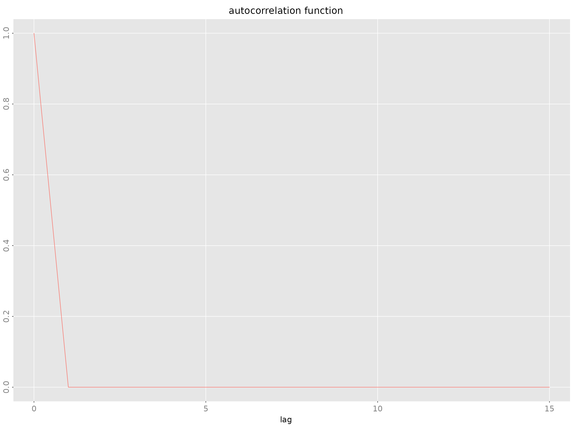

Impulse Response: impresp Class

Stores impulse response coefficients: $k_j$ where $y_t = \sum_{j \geq 0} k_j u_{t-j}$.

Structure

Slot	Type	Description
irf	array [m,n,n.lags]	IRF coefficients
sigma_L	double [n,n]	Noise covariance factor
names	character [m]	Output variable names
label	character	Descriptive label

Computation

impresp.armamod(obj, lag.max = 40, H = NULL)
impresp.stspmod(obj, lag.max = 40, H = NULL)

Example:

irf <- impresp(model, lag.max = 20)
plot(irf, main = "Impulse Response")

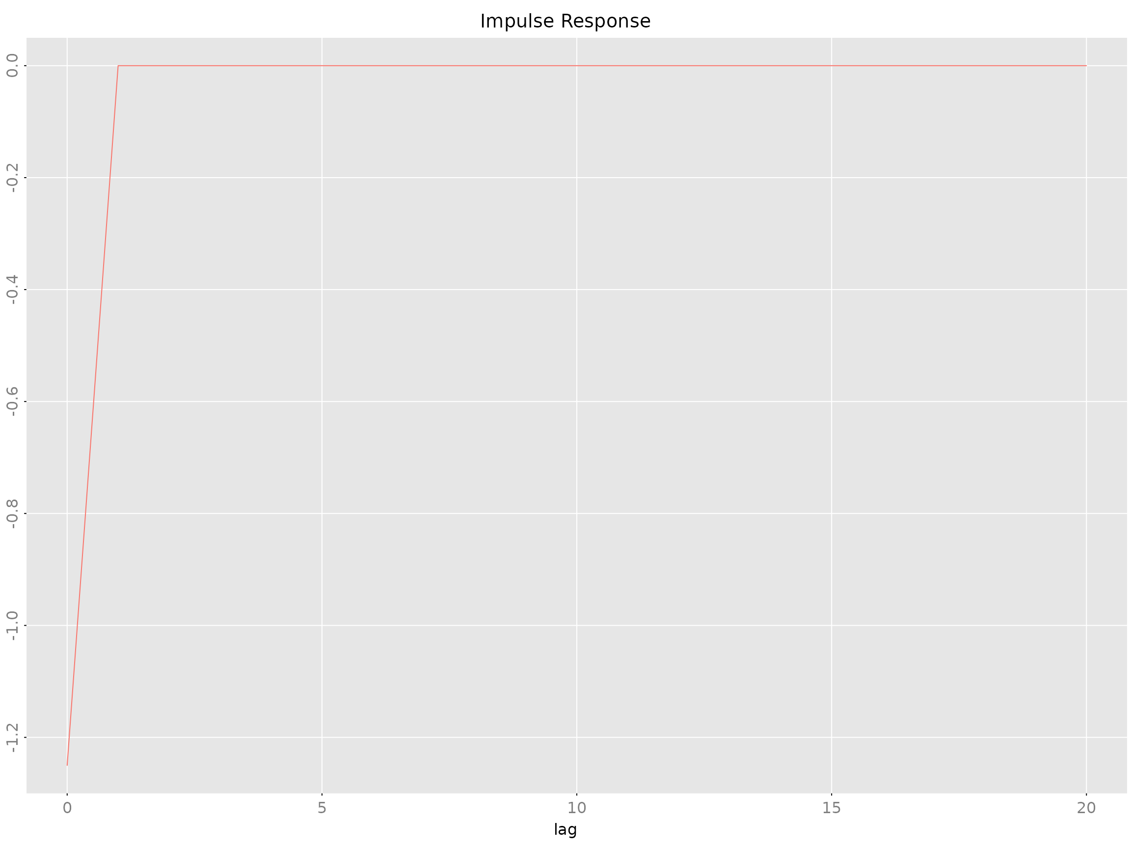
The H parameter allows custom orthogonalization (default: Cholesky).

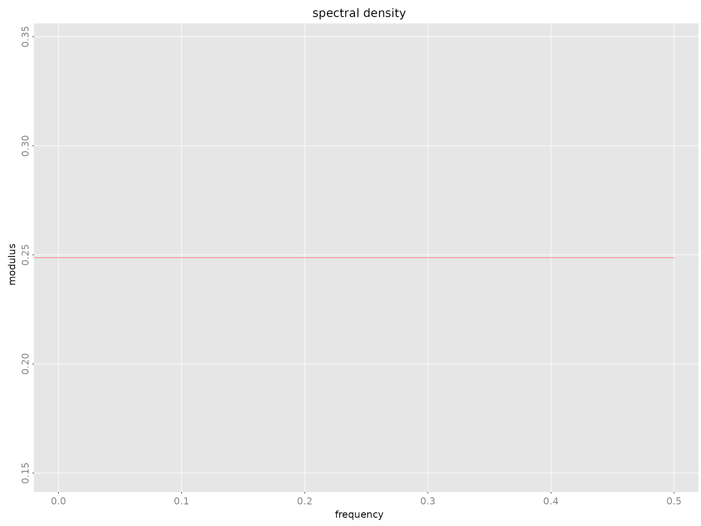
Spectral Density: spectrald Class

Frequency-domain representation: $\Gamma(\lambda) = K(\lambda) \Sigma K^*(\lambda)$ where $K(\lambda)$ is the frequency response.

Structure

Slot	Type	Description
spd	array [m,m,n.f]	Spectral density on frequency grid
names	character [m]	Variable names
label	character	Descriptive label

Computation

spectrald(obj, n.f = 128, ...)

Example:

spec <- spectrald(model, n.f = 256)
plot(spec)

Frequency Response: freqresp Class

The frequency transfer function $K(\lambda) = \sum_j k_j e^{-i\lambda j}$.

freqresp.armamod(obj, n.f = 256)

Forecast Error Variance Decomposition: fevardec Class

Decomposes forecast error variance into contributions from each shock.

Slot	Type	Description
vd	array [m,m,h]	Variance decomposition
v	matrix [m,h]	Forecast error variance
names	character [m]	Variable names

fevardec(obj, h.max = 40)

---

Estimation Methods

AR Model Estimation

Yule-Walker Method: est_ar_yw()

Theory: Solves the Yule-Walker equations using Cholesky decomposition: $$\gamma_k = a_1 \gamma_{k-1} + \cdots + a_p \gamma_{k-p}$$

Advantages: - Statistically efficient (minimum variance) - Produces all AR orders simultaneously - Automatic log-determinant sequence for model selection

Example:

est_ar_yw(gamma, p.max = 10, penalty = -1)

Durbin-Levinson-Whittle Method: est_ar_dlw()

Theory: Recursive algorithm for AR parameter and partial autocorrelation computation.

Advantages: - Numerically stable - Computes partial ACF - Efficient recursions

Example:

est_ar_dlw(gamma, p.max = 10, penalty = -1)

Wrapper Function: est_ar()

Primary interface for AR estimation with automatic order selection:

est_ar(data, p.max = NULL, method = "auto",
       ic = "AIC", mean_estimate = "sample.mean")

Parameters: - ic: Information criterion (“AIC”, “BIC”, “HQ”) - mean_estimate: How to estimate mean (“sample.mean”, “zero”, or a vector) - method: “yw” (Yule-Walker), “dlw” (Durbin-Levinson-Whittle), or “auto”

Returns: List with components: - model: Estimated armamod object - p: Selected order - stats: Criterion values for each order - ll: Log-likelihood values

---

ARMA Model Estimation

Hannan-Rissanen-Kavalieris (HRK): est_arma_hrk()

Three-stage procedure for VARMA estimation without nonlinear optimization:

est_arma_hrk(data, tmpl = NULL, p = NULL, q = NULL,
             mean_estimate = "zero")

Stage 1: Estimate long AR model Stage 2: Compute initial ARMA estimates Stage 3: Refine using feasible GLS

Advantages: - Provides consistent initial estimates - No nonlinear optimization required - Suitable for maximum likelihood refinement

When to use: - Initial estimates for multivariate ARMA - Moderate to high-dimensional systems - When you want to avoid local optima

---

State Space Estimation

CCA Method: est_stsp_ss(method = "cca")

Canonical Correlation Analysis for determining state space order and initial estimates.

est_stsp_ss(data, method = "cca", s = NULL,
            keep_models = FALSE, ...)

Advantages: - Data-driven order selection - Suitable when no prior knowledge of system structure - Good numerical properties

Subspace Methods: est_stsp_ss(method = "cca"/"ho"/"moesp")

Multiple subspace identification methods available through matrix fraction estimation.

---

Maximum Likelihood Estimation

General ML Framework: ll_FUN()

Create likelihood functions for structured parameter templates:

llfun <- ll_FUN(tmpl, data, skip = 0, which = "concentrated")

Then optimize using standard R optimizers:

out <- optim(theta0, llfun, method = "BFGS", control = list(fnscale = -1))

Parameter Templates

Templates map deep model parameters to linear parameters for optimization:

• tmpl_DDLC() - Diagonal-Direct-Lead-Coefficient
• tmpl_arma_echelon() - ARMA in echelon form
• tmpl_stsp_echelon() - State space in echelon form

Workflow:

# Create template from initial estimate
tmpl <- tmpl_DDLC(model_initial, sigma_L = 'identity')

# Extract starting parameter vector
theta0 <- extract_theta(model_initial, tmpl)

# Create and optimize likelihood
llfun <- ll_FUN(tmpl, data, which = "concentrated")
opt <- optim(theta0, llfun, method = "BFGS", control = list(fnscale = -1, maxit = 500))

# Reconstruct model from optimized parameters
model_ml <- fill_template(opt$par, tmpl)

---

Solution and Simulation

Solving Difference Equations

Forward Solution: solve_de()

Simulate forward from initial conditions:

$$y_t = k_0 u_t + k_1 u_{t-1} + k_2 u_{t-2} + \cdots$$

y <- solve_de(sys, u, y_init = NULL)

Inverse Solution: solve_inverse_de()

Extract residuals given data (solve backwards):

$$u_t = a(z)^{-1} b(z)^{-1} y_t$$

u <- solve_inverse_de(sys, y)$u

---

Mathematical Foundations

Stationary ARMA Processes

An ARMA process is described by: $$a(z) y_t = b(z) u_t$$

where: - $a(z) = I_m + a_1 z + \cdots + a_p z^p$ (AR polynomial) - $b(z) = b_0 + b_1 z + \cdots + b_q z^q$ (MA polynomial) - $(u_t)$ is white noise with $\mathbb{E}(u_t u_t') = \Sigma$

The process is stationary if all roots of $\det(a(z)) = 0$ lie outside the unit circle.

The stationary solution is: $$y_t = \sum_{j \geq 0} k_j u_{t-j}$$

where $k_j$ satisfy: $a(z) k(z) = b(z)$.

Autocovariance Function

For stationary ARMA processes, the autocovariance function $\gamma_k = \mathbb{E}(y_{t+k} y_t')$ satisfies the generalized Yule-Walker equations:

$$a_0 \gamma_k + a_1 \gamma_{k-1} + \cdots + a_p \gamma_{k-p} = \begin{cases} b_0 \Sigma k_0' + \cdots + b_q \Sigma k_{q-k}' & 0 \leq k \leq q \\ 0 & k > q \end{cases}$$

Spectral Factorization

The spectral density can be written as: $$\Gamma(\lambda) = \frac{1}{2\pi} K(\lambda) \Sigma K^*(\lambda)$$

where $K(\lambda)$ is the frequency response and $K^*$ denotes conjugate transpose.

This enables: - Frequency domain analysis - Filter design - Whitening transformations

Kronecker Indices

For VARMA models in canonical form, Kronecker indices $(n_1, \ldots, n_m)$ define the minimal orders required for each output: - Total state dimension: $s = n_1 + \cdots + n_m$ - They specify the echelon structure

---

Method Selection Guide

Choosing Between AR, ARMA, and State Space

Method	When to Use	Advantages	Disadvantages
AR	Baseline, simple systems	Fast, stable, interpretable	May need high order
ARMA	Parsimonious fits	Fewer parameters	Parameter estimation harder
State Space	Complex systems, latent factors	Flexible, interpretable states	Requires order selection

Model Comparison Workflow

1. Start with AR using est_ar()
2. Try state space with est_stsp_ss() for dimensionality reduction
3. Compare with ARMA using HRK initial estimates + ML refinement
4. Refine best model with parameter templates and optimization
5. Validate using residual diagnostics, ACF, and spectral plots

Estimation Method Selection

Task	Recommended Method
Order selection	AIC via est_ar()
Quick state space	CCA via est_stsp_ss()
Multivariate ARMA	HRK via est_arma_hrk()
Maximum likelihood	Parameter templates + optim()
Highly structured models	Custom templates with tmpl_*()

---

References

(Scherrer and Deistler 2019)

Scherrer, Wolfgang, and Manfred Deistler. 2019. “Chapter 6 - Vector Autoregressive Moving Average Models.” In Conceptual Econometrics Using r, edited by Hrishikesh D. Vinod and C. R. Rao, 41:145–91. Handbook of Statistics. Elsevier. https://doi.org/https://doi.org/10.1016/bs.host.2019.01.004.

References

- Gordon, N. J., Salmond, D. J., & Smith, A. F. M. (1993). Novel approach to nonlinear/non-Gaussian Bayesian state estimation
- Pitt, M. K., & Shephard, N. (1999). Filtering via simulation: Auxiliary particle filters
- Doucet, A., Godsill, S., & Andrieu, C. (2000). On sequential Monte Carlo sampling methods for Bayesian filtering